Zonal statistics
Quite often you have a situtation when you want to summarize raster datasets based on vector geometries. Rasterstats is a Python module that does exactly that, easily.
In [1]: import rasterio

In [2]: from rasterio.plot import show

In [3]: from rasterstats import zonal_stats

In [4]: import osmnx as ox

In [5]: import geopandas as gpd
- Specify filepath, this is the mosaic raster file that was created earlier.
In [6]: dem_fp = r"C:\HY-DATA\HENTENKA\KOODIT\Opetus\Automating-GIS-processes\Data\CSC_Lesson6\Helsinki_DEM_2x2m_Mosaic.tif"
- Read in the DEM data
In [7]: dem = rasterio.open(dem_fp)
- Specify place names for Kallio and Pihlajamäki that Nominatim can identify https://nominatim.openstreetmap.org/
In [8]: kallio_q = "Kallio, Helsinki, Finland"

In [9]: pihlajamaki_q = "Pihlajamäki, Malmi, Helsinki, Finland"
- Retrieve ‘Kallio’ and ‘Pihlajamäki’ regions from OpenStreetMap
In [10]: kallio = ox.gdf_from_place(kallio_q)

In [11]: pihlajamaki = ox.gdf_from_place(pihlajamaki_q)
- Reproject the regions to same CRS as the DEM
In [12]: kallio = kallio.to_crs(crs=dem.crs.data)

In [13]: pihlajamaki = pihlajamaki.to_crs(crs=dem.crs.data)
- Plot the DEM and the regions on top of it
In [14]: ax = show((dem, 1))
In [15]: kallio.plot(ax=ax, facecolor='None', edgecolor='red', linewidth=2)
Out[15]: <matplotlib.axes._subplots.AxesSubplot at 0x20c92beb278>
In [16]: pihlajamaki.plot(ax=ax, facecolor='None', edgecolor='blue', linewidth=2)
������������������������������������������������������������������Out[16]: <matplotlib.axes._subplots.AxesSubplot at 0x20c92beb278>
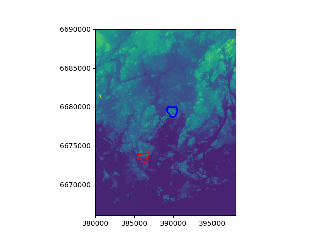
Which one is higher? Kallio or Pihlajamäki? We can use zonal statistics to find out!
- First we need to get the values of the dem as numpy array and the affine of the raster
In [17]: array = dem.read(1)

In [18]: affine = dem.affine
- Now we can calculate the zonal statistics by using the function
zonal_stats.
In [19]: zs_kallio = zonal_stats(kallio, array, affine=affine, stats=['min', 'max', 'mean', 'median', 'majority'])

In [20]: zs_pihla = zonal_stats(pihlajamaki, array, affine=affine, stats=['min', 'max', 'mean', 'median', 'majority'])
Okey. So what do we have now?
In [21]: print(zs_kallio)
[{'min': -2.1760001182556152, 'max': 37.388999938964844, 'mean': 12.96425898303966, 'median': 11.75100040435791, 'majority': 0.3490000069141388}]
In [22]: print(zs_pihla)
��������������������������������������������������������������������������������������������������������������������������������������������������[{'min': 8.73799991607666, 'max': 46.30400085449219, 'mean': 24.560033970865877, 'median': 24.17300033569336, 'majority': 10.41100025177002}]
Super! Now we can see that Pihlajamäki seems to be slightly higher compared to Kallio.