Map projections
Coordinate reference systems (CRS) are important because the geometric shapes in a GeoDataFrame are simply a collection of coordinates in an arbitrary space. A CRS tells Python how those coordinates related to places on the Earth. A map projection (or a projected coordinate system) is a systematic transformation of the latitudes and longitudes into a plain surface where units are quite commonly represented as meters (instead of decimal degrees).
As map projections of gis-layers are fairly often defined differently (i.e. they do not match), it is a common procedure to redefine the map projections to be identical in both layers. It is important that the layers have the same projection as it makes it possible to analyze the spatial relationships between layer, such as conduct the Point in Polygon spatial query.
Luckily, defining and changing projections is easy in Geopandas. In this tutorial we will see how to retrieve the coordinate reference system information from the data, and how to change it. We will re-project a data file from WGS84 (lat, lon coordinates) into a Lambert Azimuthal Equal Area projection which is the recommended projection for Europe by European Commission.
Note
Choosing an appropriate projection for your map is not always straightforward because it depends on what you actually want to represent with your map, and what is the spatial scale of your data. In fact, there does not exist a “perfect projection” since each one of them has some strengths and weaknesses, and you should choose such projection that fits best for your needs. You can read more about how to choose a map projection from here, and a nice blog post about the strengths and weaknesses of few commonly used projections.
Download data
For this tutorial we will be using a Shapefile representing Europe. Download and extract Europe_borders.zip file that contains a Shapefile with following files:
$ cd $HOME
$ unzip Europe_borders.zip
$ cd Europe_borders
$ ls
Europe_borders.cpg  Europe_borders.prj  Europe_borders.sbx  Europe_borders.shx
Europe_borders.dbf  Europe_borders.sbn  Europe_borders.shp
Coordinate reference system (CRS)
GeoDataFrame that is read from a Shapefile contains always (well not always but should) information about the coordinate system in which the data is projected.
Let’s start by reading the data from the Europe_borders.shp file.
In [1]: import geopandas as gpd

# Filepath to the Europe borders Shapefile
In [2]: fp = "/home/geo/Europe_borders.shp"

# Read data
In [3]: data = gpd.read_file(fp)
We can see the current coordinate reference system from .crs
attribute:
In [4]: data.crs
Out[4]: {'init': 'epsg:4326'}
Okey, so from this disctionary we can see that the data is something called epsg:4326. The EPSG number (“European Petroleum Survey Group”) is a code that tells about the coordinate system of the dataset. “EPSG Geodetic Parameter Dataset is a collection of definitions of coordinate reference systems and coordinate transformations which may be global, regional, national or local in application”. EPSG-number 4326 that we have here belongs to the WGS84 coordinate system (i.e. coordinates are in decimal degrees (lat, lon)).
You can find a lot of information about different available coordinate reference systems from:
Let’s also check the values in our geometry column.
In [5]: data['geometry'].head()
Out[5]:
0    POLYGON ((8.457777976989746 54.56236267089844,...
1    POLYGON ((8.71992015838623 47.69664382934571, ...
2    POLYGON ((6.733166694641113 53.5740852355957, ...
3    POLYGON ((6.858222007751465 53.59411239624024,...
4    POLYGON ((6.89894437789917 53.6256103515625, 6...
Name: geometry, dtype: object
Okey, so the coordinate values of the Polygons indeed look like lat-lon values.
Let’s convert those geometries into Lambert Azimuthal Equal Area projection (EPSG: 3035).
Changing the projection is really easy to do in Geopandas
with .to_crs() -function. As an input for the function, you
should define the column containing the geometries, i.e. geometry
in this case, and a epgs value of the projection that you want to use.
# Let's take a copy of our layer
In [6]: data_proj = data.copy()

# Reproject the geometries by replacing the values with projected ones
In [7]: data_proj = data_proj.to_crs(epsg=3035)
Let’s see how the coordinates look now.
In [8]: data_proj['geometry'].head()
Out[8]:
0    POLYGON ((4221214.558088431 3496203.404338956,...
1    POLYGON ((4224860.478308966 2732279.319617757,...
2    POLYGON ((4104652.175545862 3390034.953002084,...
3    POLYGON ((4113025.664284974 3391895.755505159,...
4    POLYGON ((4115871.227627173 3395282.099288368,...
Name: geometry, dtype: object
And here we go, the numbers have changed! Now we have successfully changed the projection of our layer into a new one, i.e. to ETRS-LAEA projection.
Note
There is also possibility to pass the projection information as proj4 strings or dictionaries, see more here
To really understand what is going on, it is good to explore our data visually. Hence, let’s compare the datasets by making maps out of them.
import matplotlib.pyplot as plt

# Plot the WGS84
data.plot(facecolor='gray');

# Add title
plt.title("WGS84 projection");

# Remove empty white space around the plot
plt.tight_layout()

# Plot the one with ETRS-LAEA projection
data_proj.plot(facecolor='blue');

# Add title
plt.title("ETRS Lambert Azimuthal Equal Area projection");

# Remove empty white space around the plot
plt.tight_layout()
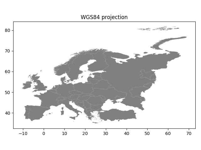
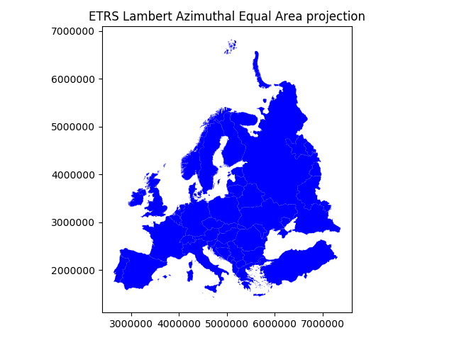
Indeed, they look quite different and our re-projected one looks much better in Europe as the areas especially in the north are more realistic and not so stretched as in WGS84.
Next, we still need to change the crs of our GeoDataFrame into EPSG
3035 as now we only modified the values of the geometry column.
We can take use of fiona’s from_epsg -function.
In [9]: from fiona.crs import from_epsg

# Determine the CRS of the GeoDataFrame
In [10]: data_proj.crs = from_epsg(3035)

# Let's see what we have
In [11]: data_proj.crs
Out[11]: {'init': 'epsg:3035', 'no_defs': True}
Finally, let’s save our projected layer into a Shapefile so that we can use it later.
# Ouput file path
outfp = r"/home/geo/Europe_borders_epsg3035.shp"

# Save to disk
data_proj.to_file(outfp)
Note
On Windows, the prj -file might NOT update with the new CRS value when using the from_epsg() -function. If this happens
it is possible to fix the prj by passing the coordinate reference information as proj4 text, like following.
In [12]: data_proj.crs = '+proj=laea +lat_0=52 +lon_0=10 +x_0=4321000 +y_0=3210000 +ellps=GRS80 +units=m +no_defs'
You can find proj4 text versions for different projection from spatialreference.org.
Each page showing spatial reference information has links for different formats for the CRS. Click a link that says Proj4 and
you will get the correct proj4 text presentation for your projection.
Alternative
PyCRS package is a handy library for dealing with projections. If you have the package installed (see installation directions), you can easily convert crs information between EPSG and ESRI codes and Proj4 specification.
We can pass the Proj4 text into GeoDataFrame as follows:
In [13]: import pycrs

In [14]: crs_info = pycrs.parser.from_epsg_code(3035)

# Now we have a CRS object
In [15]: print(crs_info)
<pycrs.elements.containers.CRS object at 0x0000020C8F837550>

# Convert to Proj4 specification string
In [16]: proj4_txt = crs_info.to_proj4()

In [17]: print(proj4_txt)
+proj=laea +ellps=GRS80 +a=6378137.0 +f=298.257222101 +pm=0  +lon_0=10 +x_0=4321000 +y_0=3210000 +lat_0=52 +units=m +axis=enu +no_defs

# Now we have a correct Proj4 text that we can pass to GeoDataFrame
In [18]: data_proj.crs = proj4_txt

# Same thing as a one-liner
In [19]: data_proj.crs = pycrs.parser.from_epsg_code(3035).to_proj4()