Introduction to Geopandas
Downloading data
For this lesson we are using data that you can download from here. Once you have downloaded the Data.zip file into your home directory, you can unzip the file using e.g. 7Zip (on Windows).
You can also use the unzip command in the Terminal window on Linux and Mac (following assumes that the file is downloaded to HOME directory:
$ cd $HOME
$ unzip Data.zip
$ ls Data
DAMSELFISH_distributions.dbf   DAMSELFISH_distributions.prj
DAMSELFISH_distributions.sbn   DAMSELFISH_distributions.sbx
DAMSELFISH_distributions.shp   DAMSELFISH_distributions.shp.xml
DAMSELFISH_distributions.shx
The Data folder includes a Shapefile called DAMSELFISH_distribution.shp (and files related to it).
Reading a Shapefile
Spatial data can be read easily with geopandas using gpd.from_file()
-function:
# Import necessary modules
In [1]: import geopandas as gpd

# Set filepath (fix path relative to yours)
In [2]: fp = "/home/geo/Data/DAMSELFISH_distributions.shp"

# Read file using gpd.read_file()
In [3]: data = gpd.read_file(fp)
- Let’s see what datatype is our ‘data’ variable
In [4]: type(data)
Out[4]: geopandas.geodataframe.GeoDataFrame
Okey so from the above we can see that our data -variable is a
GeoDataFrame. GeoDataFrame extends the functionalities of
pandas.DataFrame in a way that it is possible to use and handle
spatial data within pandas (hence the name geopandas). GeoDataFrame have
some special features and functions that are useful in GIS.
- Let’s take a look at our data and print the first 5 rows using the
head() -function prints the first 5 rows by default
In [5]: data.head()
Out[5]:
      ID_NO             BINOMIAL  ORIGIN COMPILER  YEAR  \
0  183963.0   Stegastes leucorus       1     IUCN  2010
1  183963.0   Stegastes leucorus       1     IUCN  2010
2  183963.0   Stegastes leucorus       1     IUCN  2010
3  183793.0  Chromis intercrusma       1     IUCN  2010
4  183793.0  Chromis intercrusma       1     IUCN  2010

                                            CITATION SOURCE DIST_COMM ISLAND  \
0  International Union for Conservation of Nature...   None      None   None
1  International Union for Conservation of Nature...   None      None   None
2  International Union for Conservation of Nature...   None      None   None
3  International Union for Conservation of Nature...   None      None   None
4  International Union for Conservation of Nature...   None      None   None

  SUBSPECIES                        ...                         RL_UPDATE  \
0       None                        ...                            2012.1
1       None                        ...                            2012.1
2       None                        ...                            2012.1
3       None                        ...                            2012.1
4       None                        ...                            2012.1

  KINGDOM_NA  PHYLUM_NAM      CLASS_NAME   ORDER_NAME     FAMILY_NAM  \
0   ANIMALIA    CHORDATA  ACTINOPTERYGII  PERCIFORMES  POMACENTRIDAE
1   ANIMALIA    CHORDATA  ACTINOPTERYGII  PERCIFORMES  POMACENTRIDAE
2   ANIMALIA    CHORDATA  ACTINOPTERYGII  PERCIFORMES  POMACENTRIDAE
3   ANIMALIA    CHORDATA  ACTINOPTERYGII  PERCIFORMES  POMACENTRIDAE
4   ANIMALIA    CHORDATA  ACTINOPTERYGII  PERCIFORMES  POMACENTRIDAE

  GENUS_NAME   SPECIES_NA CATEGORY  \
0  Stegastes     leucorus       VU
1  Stegastes     leucorus       VU
2  Stegastes     leucorus       VU
3    Chromis  intercrusma       LC
4    Chromis  intercrusma       LC

                                            geometry
0  POLYGON ((-115.6437454219999 29.71392059300007...
1  POLYGON ((-105.589950704 21.89339825500002, -1...
2  POLYGON ((-111.159618439 19.01535626700007, -1...
3  POLYGON ((-80.86500229899997 -0.77894492099994...
4  POLYGON ((-67.33922225599997 -55.6761029239999...

[5 rows x 24 columns]
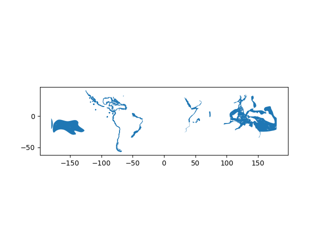
- Let’s also take a look how our data looks like on a map. If you just want to explore your data on a map, you can use
.plot()-function in geopandas that creates a simple map out of the data (uses matplotlib as a backend):
In [6]: data.plot();
Writing a Shapefile
Writing a new Shapefile is also something that is needed frequently.
- Let’s select 50 first rows of the input data and write those into a
new Shapefile by first selecting the data using index slicing and
then write the selection into a Shapefile with gpd.to_file() -function:
# Create a output path for the data
out = r"/home/geo/Data/DAMSELFISH_distributions_SELECTION.shp"

# Select first 50 rows
selection = data[0:50]

# Write those rows into a new Shapefile (the default output file format is Shapefile)
selection.to_file(out)
Task: Open the Shapefile now in QGIS that has been installed into our computer instance, and see how the data looks like.
Geometries in Geopandas
Geopandas takes advantage of Shapely’s geometric objects. Geometries are stored in a column called geometry that is a default column name for storing geometric information in geopandas.
- Let’s print the first 5 rows of the column ‘geometry’:
# It is possible to use only specific columns by specifying the column name within square brackets []
In [7]: data['geometry'].head()
Out[7]:
0    POLYGON ((-115.6437454219999 29.71392059300007...
1    POLYGON ((-105.589950704 21.89339825500002, -1...
2    POLYGON ((-111.159618439 19.01535626700007, -1...
3    POLYGON ((-80.86500229899997 -0.77894492099994...
4    POLYGON ((-67.33922225599997 -55.6761029239999...
Name: geometry, dtype: object
Since spatial data is stored as Shapely objects, it is possible to use all of the functionalities of Shapely module that we practiced earlier.
- Let’s print the areas of the first 5 polygons:
# Make a selection that contains only the first five rows
In [8]: selection = data[0:5]
We can iterate over the selected rows using a specific
.iterrows() -function in (geo)pandas and print the area for each polygon:
In [9]: for index, row in selection.iterrows():
   ...:     poly_area = row['geometry'].area
   ...:     print("Polygon area at index {0} is: {1:.3f}".format(index, poly_area))
   ...:
Polygon area at index 0 is: 19.396
Polygon area at index 1 is: 6.146
Polygon area at index 2 is: 2.697
Polygon area at index 3 is: 87.461
Polygon area at index 4 is: 0.001
Hence, as you might guess from here, all the functionalities of Pandas are available directly in Geopandas without the need to call pandas separately because Geopandas is an extension for Pandas.
- Let’s next create a new column into our GeoDataFrame where we calculate
and store the areas individual polygons. Calculating the areas of polygons is really easy in geopandas by using GeoDataFrame.area attribute:
In [10]: data['area'] = data.area
Let’s see the first 2 rows of our ‘area’ column.
In [11]: data['area'].head(2)
Out[11]:
0    19.396254
1     6.145902
Name: area, dtype: float64
Okey, so we can see that the area of our first polygon seems to be 19.39 and 6.14 for the second polygon. They correspond to the ones we saw in previous step when iterating rows, hence, everything seems to work as it should. Let’s check what is the min and the max of those areas using familiar functions from our previous Pandas lessions.
# Maximum area
In [12]: max_area = data['area'].max()

# Mean area
In [13]: mean_area = data['area'].mean()

In [14]: print("Max area: %s\nMean area: %s" % (round(max_area, 2), round(mean_area, 2)))
Max area: 1493.2
Mean area: 19.96
Okey, so the largest Polygon in our dataset seems to be 1494 square decimal degrees (~ 165 000 km2) and the average size is ~20 square decimal degrees (~2200 km2).
Creating geometries into a GeoDataFrame
Since geopandas takes advantage of Shapely geometric objects it is possible to create a Shapefile from a scratch by passing Shapely’s geometric objects into the GeoDataFrame. This is useful as it makes it easy to convert e.g. a text file that contains coordinates into a Shapefile.
Let’s create an empty GeoDataFrame.
# Import necessary modules first
import pandas as pd
import geopandas as gpd
from shapely.geometry import Point, Polygon
import fiona

# Create an empty geopandas GeoDataFrame
newdata = gpd.GeoDataFrame()
# Let's see what's inside
In [15]: newdata
Out[15]:
Empty GeoDataFrame
Columns: []
Index: []
The GeoDataFrame is empty since we haven’t placed any data inside.
Let’s create a new column called geometry that will contain our Shapely objects:
# Create a new column called 'geometry' to the GeoDataFrame
In [16]: newdata['geometry'] = None

# Let's see what's inside
In [17]: newdata
Out[17]:
Empty GeoDataFrame
Columns: [geometry]
Index: []
Now we have a geometry column in our GeoDataFrame but we don’t have any data yet.
Let’s create a Shapely Polygon repsenting the Helsinki Senate square that we can insert to our GeoDataFrame:
# Coordinates of the Helsinki Senate square in Decimal Degrees
In [18]: coordinates = [(24.950899, 60.169158), (24.953492, 60.169158), (24.953510, 60.170104), (24.950958, 60.169990)]

# Create a Shapely polygon from the coordinate-tuple list
In [19]: poly = Polygon(coordinates)

# Let's see what we have
In [20]: poly
Out[20]: <shapely.geometry.polygon.Polygon at 0x20c905ea4a8>
Okey, so now we have appropriate Polygon -object.
Let’s insert the polygon into our ‘geometry’ column in our GeoDataFrame:
# Insert the polygon into 'geometry' -column at index 0
In [21]: newdata.loc[0, 'geometry'] = poly

# Let's see what we have now
In [22]: newdata
Out[22]:
                                            geometry
0  POLYGON ((24.950899 60.169158, 24.953492 60.16...
Now we have a GeoDataFrame with Polygon that we can export to a Shapefile.
Let’s add another column to our GeoDataFrame called Location with text Senaatintori.
# Add a new column and insert data
In [23]: newdata.loc[0, 'Location'] = 'Senaatintori'

# Let's check the data
In [24]: newdata
Out[24]:
                                            geometry      Location
0  POLYGON ((24.950899 60.169158, 24.953492 60.16...  Senaatintori
Okey, now we have additional information that is useful to be able to recognice what the feature represents.
Before exporting the data it is useful to determine the coordinate reference system (projection) for the GeoDataFrame.
GeoDataFrame has a property called .crs that (more about projection on next tutorial) shows the coordinate system of the data which is empty (None) in our case since we are creating the data from the scratch:
In [25]: print(newdata.crs)
None
- Let’s add a crs for our GeoDataFrame. A Python module called
fiona has a nice function called
from_epsg()for passing coordinate system for the GeoDataFrame. Next we will use that and determine the projection to WGS84 (epsg code: 4326):
# Import specific function 'from_epsg' from fiona module
In [26]: from fiona.crs import from_epsg

# Set the GeoDataFrame's coordinate system to WGS84
In [27]: newdata.crs = from_epsg(4326)

# Let's see how the crs definition looks like
In [28]: newdata.crs
Out[28]: {'init': 'epsg:4326', 'no_defs': True}
- Finally, we can export the data using GeoDataFrames
.to_file()-function. The function works similarly as numpy or pandas, but here we only need to provide the output path for the Shapefile. Easy isn’t it!:
# Determine the output path for the Shapefile
outfp = r"/home/geo/Data/Senaatintori.shp"

# Write the data into that Shapefile
newdata.to_file(out)
Now we have successfully created a Shapefile from the scratch using only Python programming. Similar approach can be used to for example to read coordinates from a text file (e.g. points) and create Shapefiles from those automatically.
Practical example: Save multiple Shapefiles
One really useful function that can be used in Pandas/Geopandas is .groupby(). We saw and used this function already in Lesson 5 of the Geo-Python course. Group by function is useful to group data based on values on selected column(s).
- Let’s group individual fishes in
DAMSELFISH_distribution.shpand export the species to individual Shapefiles.- Note: If your `data` -variable doesn’t contain the Damselfish data anymore, read the Shapefile again into memory using `gpd.read_file()` -function
# Group the data by column 'BINOMIAL'
In [29]: grouped = data.groupby('BINOMIAL')

# Let's see what we got
In [30]: grouped
Out[30]: <pandas.core.groupby.DataFrameGroupBy object at 0x0000020C8F3E9048>
groupby-function gives us an object calledDataFrameGroupBywhich is similar to list of keys and values (in a dictionary) that we can iterate over.
# Iterate over the group object
In [31]: for key, values in grouped:
   ....:     individual_fish = values
   ....:

# Let's see what is the LAST item that we iterated
In [32]: individual_fish
Out[32]:
       ID_NO                BINOMIAL  ORIGIN COMPILER  YEAR  \
27  154915.0  Teixeirichthys jordani       1     None  2012
28  154915.0  Teixeirichthys jordani       1     None  2012
29  154915.0  Teixeirichthys jordani       1     None  2012
30  154915.0  Teixeirichthys jordani       1     None  2012
31  154915.0  Teixeirichthys jordani       1     None  2012
32  154915.0  Teixeirichthys jordani       1     None  2012
33  154915.0  Teixeirichthys jordani       1     None  2012

                                             CITATION SOURCE DIST_COMM ISLAND  \
27  Red List Index (Sampled Approach), Zoological ...   None      None   None
28  Red List Index (Sampled Approach), Zoological ...   None      None   None
29  Red List Index (Sampled Approach), Zoological ...   None      None   None
30  Red List Index (Sampled Approach), Zoological ...   None      None   None
31  Red List Index (Sampled Approach), Zoological ...   None      None   None
32  Red List Index (Sampled Approach), Zoological ...   None      None   None
33  Red List Index (Sampled Approach), Zoological ...   None      None   None

   SUBSPECIES    ...     KINGDOM_NA PHYLUM_NAM      CLASS_NAME   ORDER_NAME  \
27       None    ...       ANIMALIA   CHORDATA  ACTINOPTERYGII  PERCIFORMES
28       None    ...       ANIMALIA   CHORDATA  ACTINOPTERYGII  PERCIFORMES
29       None    ...       ANIMALIA   CHORDATA  ACTINOPTERYGII  PERCIFORMES
30       None    ...       ANIMALIA   CHORDATA  ACTINOPTERYGII  PERCIFORMES
31       None    ...       ANIMALIA   CHORDATA  ACTINOPTERYGII  PERCIFORMES
32       None    ...       ANIMALIA   CHORDATA  ACTINOPTERYGII  PERCIFORMES
33       None    ...       ANIMALIA   CHORDATA  ACTINOPTERYGII  PERCIFORMES

       FAMILY_NAM      GENUS_NAME SPECIES_NA CATEGORY  \
27  POMACENTRIDAE  Teixeirichthys    jordani       LC
28  POMACENTRIDAE  Teixeirichthys    jordani       LC
29  POMACENTRIDAE  Teixeirichthys    jordani       LC
30  POMACENTRIDAE  Teixeirichthys    jordani       LC
31  POMACENTRIDAE  Teixeirichthys    jordani       LC
32  POMACENTRIDAE  Teixeirichthys    jordani       LC
33  POMACENTRIDAE  Teixeirichthys    jordani       LC

                                             geometry       area
27  POLYGON ((121.6300326400001 33.04248618400004,...  38.671198
28  POLYGON ((32.56219482400007 29.97488975500005,...  37.445735
29  POLYGON ((130.9052090560001 34.02498196400006,...  16.939460
30  POLYGON ((56.32233070000007 -3.707270205999976...  10.126967
31  POLYGON ((40.64476131800006 -10.85502363999996...   7.760303
32  POLYGON ((48.11258402900006 -9.335103113999935...   3.434236
33  POLYGON ((51.75403543100003 -9.21679305899994,...   2.408620

[7 rows x 25 columns]
From here we can see that an individual_fish variable now contains all the rows that belongs to a fish called Teixeirichthys jordani. Notice that the index numbers refer to the row numbers in the
original data -GeoDataFrame.
- Let’s check the datatype of the grouped object and what does the
keyvariable contain
In [33]: type(individual_fish)
Out[33]: geopandas.geodataframe.GeoDataFrame
In [34]: print(key)
���������������������������������������������Teixeirichthys jordani
As can be seen from the example above, each set of data are now grouped into separate GeoDataFrames that we can export into Shapefiles using the variable key
for creating the output filepath names. Here we use a specific string formatting method to produce the output filename using % operator (read more here).
Let’s now export those species into individual Shapefiles.
# Determine outputpath
outFolder = r"/home/geo/Data"

# Create a new folder called 'Results' (if does not exist) to that folder using os.makedirs() function
resultFolder = os.path.join(outFolder, 'Results')
if not os.path.exists(resultFolder):
    os.makedirs(resultFolder)

# Iterate over the
for key, values in grouped:
    # Format the filename (replace spaces with underscores)
    outName = "%s.shp" % key.replace(" ", "_")

    # Print some information for the user
    print("Processing: %s" % key)

    # Create an output path
    outpath = os.path.join(resultFolder, outName)

    # Export the data
    values.to_file(outpath)
Now we have saved those individual fishes into separate Shapefiles and named the file according to the species name. These kind of grouping operations can be really handy when dealing with Shapefiles. Doing similar process manually would be really laborious and error-prone.