Retrieving OpenStreetMap data¶

What is OpenStreetMap?¶

OpenStreetMap (OSM) is a global collaborative (crowd-sourced) dataset and project that aims at creating a free editable map of the world containing a lot of information about our environment. It contains data for example about streets, buildings, different services, and landuse to mention a few.

OSM has a large userbase with more than 4 million users that contribute actively on OSM by updating the OSM database with 3 million changesets per day. In total OSM contains more than 4 billion nodes that form the basis of the digitally mapped world that OSM provides (stats from November 2017.

OpenStreetMap is used not only for integrating the OSM maps as background maps to visualizations or online maps, but also for many other purposes such as routing, geocoding, education, and research. OSM is also widely used for humanitarian response e.g. in crisis areas (e.g. after natural disasters) and for fostering economic development (see more from Humanitarian OpenStreetMap Team (HOTOSM) website.

Osmnx¶

This week we will explore a new and exciting Python module called osmnx that can be used to retrieve, construct, analyze, and visualize street networks from OpenStreetMap. In short it offers really handy functions to download data from OpenStreet map, analyze the properties of the OSM street networks, and conduct network routing based on walking, cycling or driving.

There is also a scientific article available describing the package:

Boeing, G. 2017. “OSMnx: New Methods for Acquiring, Constructing, Analyzing, and Visualizing Complex Street Networks.” Computers, Environment and Urban Systems 65, 126-139. doi:10.1016/j.compenvurbsys.2017.05.004

Download and visualize OpenStreetMap data with osmnx¶

As said, one the most useful features that osmnx provides is an easy-to-use way of retrieving OpenStreetMap data (using OverPass API ).

Let’s see how we can download and visualize street network data from a district of Kamppi in Helsinki, Finland. Osmnx makes it really easy to do that as it allows you to specify an address to retrieve the OpenStreetMap data around that area. In fact, osmnx uses the same Nominatim Geocoding API to achieve this which we tested during the Lesson 2.

Let’s retrieve OpenStreetMap (OSM) data by specifying "Kamppi, Helsinki, Finland" as the address where the data should be downloaded.

In [1]: import osmnx as ox

In [2]: import matplotlib.pyplot as plt

In [3]: place_name = "Kamppi, Helsinki, Finland"

In [4]: graph = ox.graph_from_place(place_name)

In [5]: type(graph)
Out[5]: networkx.classes.multidigraph.MultiDiGraph

Okey, as we can see the data that we retrieved is a special data object called networkx.classes.multidigraph.MultiDiGraph. A DiGraph is a data type that stores nodes and edges with optional data, or attributes. What we can see here is that this data type belongs to a Python module called networkx that can be used to create, manipulate, and study the structure, dynamics, and functions of complex networks. Networkx module contains algorithms that can be used to calculate shortest paths along networks using e.g. Dijkstra’s or A* algorithm.

Let’s see how our street network looks like. It is easy to visualize the graph with osmnx with plot_graph() function. The function utilizes Matplotlib for visualizing the data,

hence as a result it returns a matplotlib figure and axis objects.

In [6]: fig, ax = ox.plot_graph(graph)

In [7]: plt.tight_layout()

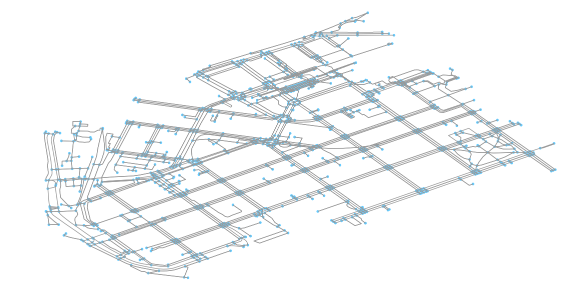
Great! Now we can see that our graph contains the nodes (blue circles) and the edges (gray lines) that connects those nodes to each other.

It is also possible to retrieve other types of OSM data features with osmnx.

Let’s download the buildings with buildings_from_place() function and plot them on top of our street network in Kamppi. Let’s also plot the Polygon that represents the area of Kamppi,

Helsinki that can be retrieved with gdf_from_place function.

In [8]: area = ox.gdf_from_place(place_name)

In [9]: buildings = ox.buildings_from_place(place_name)

In [10]: type(area)
Out[10]: geopandas.geodataframe.GeoDataFrame

In [11]: type(buildings)
Out[11]: geopandas.geodataframe.GeoDataFrame

As a result we got the data as GeoDataFrames. Hence, we can plot them using the familiar plot() function of Geopandas. As you might remember the street network data was not in GeoDataFrame. Luckily, osmnx provides a convenient function graph_to_gdfs() that can convert the graph into two separate GeoDataFrames where the first one contains the information about the nodes and the second one about the edges.

Let’s extract the nodes and edges from the graph as GeoDataFrames.

In [12]: nodes, edges = ox.graph_to_gdfs(graph)

In [13]: nodes.head()
Out[13]: 
           highway     osmid   ref        x        y  \
25216594       NaN  25216594   NaN   24.921  60.1648   
25238874       NaN  25238874   NaN   24.921  60.1637   
25238883  crossing  25238883   NaN  24.9214  60.1634   
25238933  bus_stop  25238933  1168  24.9245  60.1611   
25238944       NaN  25238944   NaN  24.9213  60.1646   

                               geometry  
25216594  POINT (24.9209884 60.1647959)  
25238874  POINT (24.9210331 60.1636625)  
25238883  POINT (24.9214283 60.1634425)  
25238933   POINT (24.924529 60.1611136)  
25238944   POINT (24.921303 60.1646301)  

In [14]: edges.head()
Out[14]: 
  access bridge                                           geometry   highway  \
0    NaN    NaN  LINESTRING (24.9209884 60.1647959, 24.9208687 ...   primary   
1    NaN    NaN  LINESTRING (24.9209884 60.1647959, 24.9209472 ...   primary   
2    NaN    NaN  LINESTRING (24.9210331 60.1636625, 24.9210408 ...   primary   
3    NaN    NaN  LINESTRING (24.9214283 60.1634425, 24.9214018 ...   primary   
4    NaN    NaN  LINESTRING (24.9214283 60.1634425, 24.9210916 ...  cycleway   

   key lanes     length maxspeed            name  oneway  \
0    0     2   6.654290       40   Porkkalankatu    True   
1    0     2  40.546678       40  Mechelininkatu    True   
2    0     2   5.597971       40  Mechelininkatu    True   
3    0     4  16.322546       40  Mechelininkatu    True   
4    0   NaN  18.647504      NaN             NaN   False   

                  osmid service tunnel         u           v  
0              23717777     NaN    NaN  25216594  1372425721  
1  [23856784, 31503767]     NaN    NaN  25216594  1372425714  
2              29977177     NaN    NaN  25238874   336192701  
3              58077048     NaN    NaN  25238883   568147264  
4             160174209     NaN    NaN  25238883   258190363  

In [15]: type(edges)
Out[15]: geopandas.geodataframe.GeoDataFrame

Nice! Now, as we can see, we have our graph as GeoDataFrames and we can plot them using the same functions and tools as we have used before.

Note

There are also other ways of retrieving the data from OpenStreetMap with osmnx such as passing a Polygon to extract the data from that area, or passing a Point coordinates and retrieving data around that location with specific radius. Take a look of this tutorial to find out how to use those features of osmnx.

Let’s create a map out of the streets, buildings, and the area Polygon but let’s exclude the nodes (to keep the figure clearer).

In [16]: fig, ax = plt.subplots()

In [17]: area.plot(ax=ax, facecolor='black')
Out[17]: <matplotlib.axes._subplots.AxesSubplot at 0x2ce1cdad940>

In [18]: edges.plot(ax=ax, linewidth=1, edgecolor='#BC8F8F')
Out[18]: <matplotlib.axes._subplots.AxesSubplot at 0x2ce1cdad940>

In [19]: buildings.plot(ax=ax, facecolor='khaki', alpha=0.7)
Out[19]: <matplotlib.axes._subplots.AxesSubplot at 0x2ce1cdad940>

In [20]: plt.tight_layout()

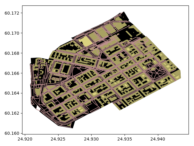
Cool! Now we have a map where we have plotted the buildings, streets and the boundaries of the selected region of ‘Kamppi’ in Helsinki. And all of this required only a few lines of code. Pretty neat! Next, we will start exploring how we can use OSM data to do network analysis.

Todo

Task Column highway in our edges GeoDataFrame contains information about the type of the street (such as primacy, cycleway or footway). Select the streets that are walkable or that can be used with cycle and visualize only them with the buildings and the area polygon. Use different colors and line widths for the cycleways and footways.

Hint

There are a few nice and convenient high-level functions in osmnx that can be used to produce nice maps directly just by using a single function that might be useful. If you are interested take a look of this tutorial. In the lesson we won’t cover these, because we wanted to keep as much control to ourselves as possible, hence using lower-level functions.