Processing toolbox scripts
Managing and organising complex composite algorithms in the Graphical Modeler is not only tedious, it also only offers very limited logic operations. For more flexible and more advanced algorithms, the processing toolbox allows to implement python scripts. A python script integrated into the processing toolbox can access all of processing’s algorithms and its user interface, the entire python application programming interface (API) of QGIS (see. the PyQGIS Developer Cookbook), and any other python module installed in the same python environment QGIS is running it.
Note
Python and its ecosystem are highly modular. It is not uncommon to find multiple python installations on a single computer. Many applications require specific versions of python and/or some of its modules. For developers of python-dependent software, it has become common to supply a requirements.txt file which can be used to initialise a so-called virtual environment, using tools such as (ana)conda.
On Microsoft Windows, unfortunately most programs ship with their private python enviroment which is difficult to access outside of the respective program and even harder to install additional packages into. For instance, ESRI ArcGIS and QGIS use entirely separate python installations. On Linux and macOS, QGIS typically uses the system python environment, but QGIS’ own packages are per-default only accessible from within the program.
To add a new python script to the processing toolbox, choose Scripts → Tools → Create new script from the toolbox. It is advisable to try the script in the interactive IPyConsole first, though.
Processing in the IPython console
Note
In this course, we use the soon-to-be-released next major QGIS version, 3.0. There have been major changes in QGIS, one of them being a complete rewrite of the processing API. At the time of this writing, documentation is still incomplete.
Import the processing module to use its algorithms:
import processing
Previous to QGIS 2.99, processing offered a processing.alglist() command to list all available algorithms and search for keywords in their names. In QGIS 3.0, the following two lines are an easy drop-in for the same search:
# search for “buffer” algorithms:
In [1]: searchTerm = "buffer"
In [2]: print([a.id() for a in QgsApplication.processingRegistry().algorithms() if searchTerm in a.id()])
Out[2]:
    ['gdal:buffervectors',
     'gdal:onesidebuffer',
     'grass7:r.buffer',
     'grass7:r.buffer.lowmem',
     'grass7:v.buffer.column',
     'grass7:v.buffer.distance',
     'native:buffer',
     'qgis:fixeddistancebuffer',
     'qgis:singlesidedbuffer',
     'qgis:variabledistancebuffer']
Note
This code uses a very pythonic programming language feature: list comprehensions. A list is a variable containing zero, one or more values, in the order they were added to the list. To define a list, put its member values (if any) inside brackets, comma-separated: ["a", "list", "of", "strings"]. In the above example, the list is filled with values created on-the-fly in a for-loop within these brackets. (List comprehension is an advanced language feature, and copy-&-paste is fine for the purpose of this course)
To access more information on an individual algorithm, run processing.algorithmHelp():
In [3]: processing.algorithmHelp("native:buffer")
Out[3]:
    Buffer (native:buffer)

    This algorithm computes a buffer area for all the features in an input layer, using a fixed or dynamic distance.

    The segments parameter controls the number of line segments to use to approximate a quarter circle when creating rounded offsets.

    The end cap style parameter controls how line endings are handled in the buffer.

    The join style parameter specifies whether round, miter or beveled joins should be used when offsetting corners in a line.

    The miter limit parameter is only applicable for miter join styles, and controls the maximum distance from the offset curve to use when creating a mitered join.

    ----------------
    Input parameters
    ----------------

    INPUT:  <QgsProcessingParameterFeatureSource>
            Input layer

    DISTANCE:  <QgsProcessingParameterNumber>
            Distance

    SEGMENTS:  <QgsProcessingParameterNumber>
            Segments

    END_CAP_STYLE:  <QgsProcessingParameterEnum>
            End cap style
                    0 - Round
                    1 - Flat
                    2 - Square

    JOIN_STYLE:  <QgsProcessingParameterEnum>
            Join style
                    0 - Round
                    1 - Miter
                    2 - Bevel

    MITER_LIMIT:  <QgsProcessingParameterNumber>
            Miter limit

    DISSOLVE:  <QgsProcessingParameterBoolean>
            Dissolve result

    OUTPUT:  <QgsProcessingParameterFeatureSink>
            Buffered

    ----------------
    Outputs
    ----------------

    OUTPUT:  <QgsProcessingOutputVectorLayer>
            Buffered
Rasterise Species Range Maps
We want to create a script which for our example damselfish dataset or any similar dataset loops over the described species, and exports one raster dataset per species, containing its respective species range map.
Let’s develop the script in the IPython console. Because at this stage we don’t run this script from within processing, we have to import processing manually, and manually define the input variables which will later be taken from the toolbox menu. (Make sure you have the damselfish data loaded.)
import os.path
import processing

# define variables manually (hard-coded),
# only for script development on the console
# (replaced later)

# input layer
Species_Range_Polygons = iface.activeLayer()
# species column name
Species_Attribute = "BINOMIAL"
# column name to be added and rasterised
Presence_Field_Name = "presence"
# value for this column (and the later raster values)
Presence_Field_Value = 1
# output directory
Output_Directory = "/tmp"
The variable names are already prepared for later saving this script as a processing script. The variable names are cleaned (underscore is replaced by space) and used for labelling the input user interface. Thus, a variable name of Species_Range_Polygons will result in an input field labelled “Species Range Polygons”.
Adding a new field and updating its value
We need to add a new field with a user-defined name. This field name is stored in Presence_Field_Name. We use the field calculator algorithm of the processing toolbox. To find its scripting name (id), search for it, then display its help text:
# search for “buffer” algorithms:
In [3]: searchTerm = "calculator"
In [4]: print([a.id() for a in QgsApplication.processingRegistry().algorithms() if searchTerm in a.id()])
Out[4]: ['qgis:advancedpythonfieldcalculator', 'qgis:fieldcalculator', 'qgis:rastercalculator']
In [5]: processing.algorithmHelp
Out[5]: Field calculator (qgis:fieldcalculator)

This algorithm computes a new vector layer with the same features of the input layer, but with an additional attribute. The values of this new attribute are computed from each feature using a mathematical formula, based on the properties and attributes of the feature.


----------------
Input parameters
----------------

INPUT:  <QgsProcessingParameterFeatureSource>
        Input layer

FIELD_NAME:  <QgsProcessingParameterString>
        Result field name

FIELD_TYPE:  <QgsProcessingParameterEnum>
        Field type
                0 - Float
                1 - Integer
                2 - String
                3 - Date

FIELD_LENGTH:  <QgsProcessingParameterNumber>
        Field length

FIELD_PRECISION:  <QgsProcessingParameterNumber>
        Field precision

NEW_FIELD:  <QgsProcessingParameterBoolean>
        Create new field

FORMULA:  <QgsProcessingParameterExpression>
        Formula

OUTPUT:  <QgsProcessingParameterFeatureSink>
        Calculated

----------------
Outputs
----------------

OUTPUT:  <QgsProcessingOutputVectorLayer>
        Calculated
We use processing.run() to run the algorithm, and have to supply the algorithm’s id and all input parameters in a dictionary. run() returns a dictionary with all output values, amongst them the output layer.
algorithmOutput = processing.run(
    "qgis:fieldcalculator",
    {
        "INPUT": Species_Range_Polygons,
        "FIELD_NAME": Presence_Field_Name,
        "FIELD_TYPE": 1,
        "FIELD_LENGTH": 5,
        "FIELD_PRECISION": 0,
        "NEW_FIELD": True,
        "FORMULA": Presence_Field_Value,
        "OUTPUT": "memory:speciesRangePolygonsWithPresenceValue"
    }
)
speciesRangePolygonsWithPresenceValue = algorithmOutput["OUTPUT"]
Finding unique species
As we wanted to save individual species into separate raster files, we need to determine the unique species in our attribute table. For this, we will use the layer’s uniqueValues() function, which requires a field’s index instead of its name. This function is somewhat equivalent to Geopandas unique().
# get the field index for the column "Species_Attribute"
fields = speciesRangePolygonsWithPresenceValue.fields()
fieldIndex = fields.indexFromName(Species_Attribute)

# get unique values for this columns
uniqueSpecies = Species_Range_Polygons.uniqueValues(fieldIndex)
Select by attribute and rasterise
Now, for each species we run three algorithms: we use select by attribute (qgis:selectbyattribute) to save the features belonging to the current species into a new layer. Because the rasterize algorithm does not understand the default in-memory vector file format, we write the vector data to an intermediate file and then convert the vector data into a raster file using the rasterize (vector to raster) tool (gdal:rasterize). Before that, we have to define an output file name for our raster.
# loop over unique species
for species in uniqueSpecies:
    # define output raster file name:
    outputFile = os.path.join(
        Output_Directory,
        species.replace(" ","_")
    )

    # select only feature with the current species
    algorithmOutput = processing.run(
        "qgis:selectbyattribute",
        {
            "INPUT": speciesRangePolygonsWithPresenceValue,
            "FIELD": Species_Attribute,
            "OPERATOR": 0,
            "VALUE": species
        }
    )
    oneSpeciesRangePolygons = algorithmOutput["OUTPUT"]

    # save intermediate vector file
    algorithmOutput = processing.run(
        "native:saveselectedfeatures",
        {
            "INPUT": oneSpeciesRangePolygons,
            "OUTPUT": outputFile + ".shp"
        }
    )
    oneSpeciesRangePolygons = algorithmOutput["OUTPUT"]

    # rasterise the vector layer
    algorithmOutput = processing.run(
        "gdal:rasterize",
        {
            "INPUT": oneSpeciesRangePolygons,
            "FIELD": Presence_Field_Name,
            "DIMENSIONS": 0,
            "WIDTH": 2000,
            "HEIGHT": 1000,
            "RAST_EXT": "",
            "RTYPE": 0,
            "OUTPUT": outputFile + ".tif"
        }
    )
Adding the script to the toolbox
After developing the script in the IPython console, let’s create a proper processing toolbox script. Open the processing script editor (Scripts → Tools → Create new script in the toolbox) and paste the code. Save it in the default directory.
The only changes are in the very top of the file: we have to add metadata to describe which parameters our script accepts, plus its name and category. The syntax for this information is ##[Variable name]=[Variable type] [optional default value and/or type]. Valid variable types include vector and raster, number and string and a view more. Find a more complete list in the QGIS user manual. Finally, there is name and group.
##Rasterize Species Range Maps=name
##Conservation Geography=group
##Species_Range_Polygons=vector polygon
##Species_Attribute=field Species_Range_Polygons
##Presence_Field_Name=string presence
##Presence_Field_Value=expression 1
##Output_Directory=folder /tmp/
Run the script
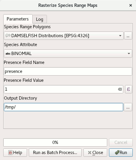
To run the script, find it from the toolbox, select DAMSELFISH Distributions as the input layer, BINOMIAL as the species attribute, and specify an output directory. Then click Run.
The full script
##Rasterize Species Range Maps=name
##Conservation Geography=group
##Species_Range_Polygons=vector polygon
##Species_Attribute=field Species_Range_Polygons
##Presence_Field_Name=string presence
##Presence_Field_Value=expression 1
##Output_Directory=folder /tmp/


import os.path


algorithmOutput = processing.run(
    "qgis:fieldcalculator",
    {
        "INPUT": Species_Range_Polygons,
        "FIELD_NAME": Presence_Field_Name,
        "FIELD_TYPE": 1,
        "FIELD_LENGTH": 5,
        "FIELD_PRECISION": 0,
        "NEW_FIELD": True,
        "FORMULA": Presence_Field_Value,
        "OUTPUT": "memory:speciesRangePolygonsWithPresenceValue"
    }
)
speciesRangePolygonsWithPresenceValue = algorithmOutput["OUTPUT"]

# get the field index for the column "Species_Attribute"
fields = speciesRangePolygonsWithPresenceValue.fields()
fieldIndex = fields.indexFromName(Species_Attribute)

# get unique values for this columns
uniqueSpecies = Species_Range_Polygons.uniqueValues(fieldIndex)

# loop over unique species
for species in uniqueSpecies:

    # define output file name:
    outputFile = os.path.join(
        Output_Directory,
        species.replace(" ","_")
    )

    # select only feature with the current species
    algorithmOutput = processing.run(
        "qgis:selectbyattribute",
        {
            "INPUT": speciesRangePolygonsWithPresenceValue,
            "FIELD": Species_Attribute,
            "OPERATOR": 0,
            "VALUE": species
        }
    )
    oneSpeciesRangePolygons = algorithmOutput["OUTPUT"]

    # save intermediate vector file
    algorithmOutput = processing.run(
        "native:saveselectedfeatures",
        {
            "INPUT": oneSpeciesRangePolygons,
            "OUTPUT": outputFile + ".shp"
        }
    )
    oneSpeciesRangePolygons = algorithmOutput["OUTPUT"]

    # rasterise the vector layer
    algorithmOutput = processing.run(
        "gdal:rasterize",
        {
            "INPUT": oneSpeciesRangePolygons,
            "FIELD": Presence_Field_Name,
            "DIMENSIONS": 0,
            "WIDTH": 2000,
            "HEIGHT": 1000,
            "RAST_EXT": "",
            "RTYPE": 0,
            "OUTPUT": outputFile + ".tif"
        }
    )