Geometric operations
Overlay analysis
The aim here is to make an overlay analysis where we select only specific polygon cells from the data based on the borders of municipality of Helsinki.
Let’s first read the data.
import geopandas as gpd
import matplotlib.pyplot as plt
import shapely.speedups

# Let's enable speedups to make queries faster
shapely.speedups.enable()

# File paths
border_fp = "/home/geo/data/Helsinki_borders.shp"
grid_fp = "/home/geo/data/TravelTimes_to_5975375_RailwayStation.shp"

# Read files
grid = gpd.read_file(grid_fp)
hel = gpd.read_file(border_fp)
Let’s check that the coordinate systems match.
In [1]: hel.crs
Out[1]: {'init': 'epsg:3067'}
In [2]: grid.crs
������������������������������Out[2]: {'init': 'epsg:3067'}
Indeed, they do. This is pre-srequisite to conduct spatial operations between the layers (as their coordinates need to match).
Let’s see how our datasets look like. We will use the Helsinki municipality layer as our basemap and plot the other layer on top of that.
In [3]: basemap = hel.plot()

In [4]: grid.plot(ax=basemap, facecolor='gray' linewidth=0.02);

# Use tight layout
Let’s do an overlay analysis and select polygons from grid that intersect with our Helsinki layer.
Note
This can be a slow procedure with less powerful computer. There is a way to overcome this issue by doing the analysis in batches which is explained below, see the performance-tip.
In [5]: result = gpd.overlay(grid, hel, how='intersection')
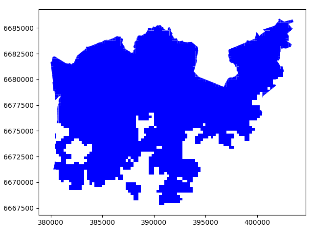
Let’s plot our data and see what we have.
In [6]: result.plot(color="b")
Out[6]: <matplotlib.axes._subplots.AxesSubplot at 0x2ce1cb682b0>

In [7]: plt.tight_layout()

Cool! Now as a result we have only those grid cells included that intersect with the Helsinki borders and the grid cells are clipped based on the boundary.
Whatabout the data attributes? Let’s see what we have.
In [8]: result.head()
Out[8]:
   car_m_d  car_m_t  car_r_d  car_r_t  from_id  pt_m_d  pt_m_t  pt_m_tt  \
0    15981       36    15988       41  6002702   14698      65       73
1    16190       34    16197       39  6002701   14661      64       73
2    15727       33    15733       37  6001132   14256      59       69
3    15975       33    15982       37  6001131   14512      62       73
4    16136       35    16143       40  6001138   14730      65       73

   pt_r_d  pt_r_t  pt_r_tt    to_id  walk_d  walk_t    GML_ID   NAMEFIN  \
0   14698      61       72  5975375   14456     207  27517366  Helsinki
1   14661      60       72  5975375   14419     206  27517366  Helsinki
2   14256      55       62  5975375   14014     200  27517366  Helsinki
3   14512      58       70  5975375   14270     204  27517366  Helsinki
4   14730      61       72  5975375   14212     203  27517366  Helsinki

       NAMESWE NATCODE                                           geometry
0  Helsingfors     091  POLYGON ((391000.0001349226 6667750.00004299, ...
1  Helsingfors     091  POLYGON ((390750.0001349644 6668000.000042951,...
2  Helsingfors     091  POLYGON ((391000.0001349143 6668000.000042943,...
3  Helsingfors     091  POLYGON ((390750.0001349644 6668000.000042951,...
4  Helsingfors     091  POLYGON ((392500.0001346234 6668000.000042901,...
Nice! Now we have attributes from both layers included.
Let’s see the length of the GeoDataFrame.
In [9]: len(result)
Out[9]: 3836
And the original data.
In [10]: len(grid)
Out[10]: 13231
Let’s save our result grid as a GeoJSON file that is another commonly used file format nowadays for storing spatial data.
resultfp = "/home/geo/data/TravelTimes_to_5975375_RailwayStation_Helsinki.geojson"

# Use GeoJSON driver
result.to_file(resultfp, driver="GeoJSON")
There are many more examples for different types of overlay analysis in Geopandas documentation where you can go and learn more.
Hint
Overlay analysis such as ours with around 13 000 polygons is quite CPU intensive task which can be quite slow to execute. Luckily, doing such analysis in batches improves the performance dramatically (spatial lookups are much quicker that way). The code snippet below shows how to do it with batch size of 10 rows which takes only around 1.5 minutes to run the analysis in our computer instance.
import geopandas as gpd
import numpy as np

# File paths
border_fp = "/home/geo/data/Helsinki_borders.shp"
grid_fp = "/home/geo/data/TravelTimes_to_5975375_RailwayStation.shp"

# Read files
grid = gpd.read_file(grid_fp)
hel = gpd.read_file(border_fp)

# Batch size
b = 10

# Number of iterations (round up with np.ceil) and convert to integer
row_cnt = len(grid)
iterations = int(np.ceil(row_cnt / b))

# Final result
final = gpd.GeoDataFrame()

# Set the start and end index according the batch size
start_idx = 0
end_idx = start_idx + b

for iteration in range(iterations):
    print("Iteration: %s/%s" % (iteration, iterations))

    # Make an overlay analysis using a subset of the rows
    result = gpd.overlay(grid[start_idx:end_idx], hel, how='intersection')

    # Append the overlay result to final GeoDataFrame
    final = final.append(result)

    # Update indices
    start_idx += b
    end_idx = start_idx + b

# Save the output as GeoJSON
outfp = "/home/geo/data/overlay_analysis_speedtest.geojson"
final.to_file(outfp, driver="GeoJSON")
Aggregating data
Aggregating data can also be useful sometimes. What we mean by aggregation is that we basically merge Geometries into together by some common identifier. Suppose we are interested in studying continents, but we only have country-level data like the country dataset. By aggregation we would convert this into a continent-level dataset.
Let’s aggregate our travel time data by car travel times, i.e. the grid cells that have the same travel time to Railway Station will be merged together.
In [11]: result_aggregated = result.dissolve(by="car_r_t")

In [12]: result_aggregated.head()
Out[12]:
                                                  geometry  car_m_d  car_m_t  \
car_r_t
-1       (POLYGON ((388000.0001354737 6669000.000042855...       -1       -1
 0       POLYGON ((386000.0001357812 6672000.000042388,...        0        0
 7       POLYGON ((386250.0001357396 6671750.000042424,...     1059        7
 8       (POLYGON ((386250.0001357467 6671500.000042468...     1207        8
 9       (POLYGON ((387000.0001355996 6671500.000042449...     1768        8

         car_r_d  from_id  pt_m_d  pt_m_t  pt_m_tt  pt_r_d  pt_r_t  pt_r_tt  \
car_r_t
-1            -1  5996387      -1      -1       -1      -1      -1       -1
 0             0  5975375       0       0        0       0       0        0
 7          1059  5977007     447       6        6     447       6        6
 8          1207  5978638    1026       9       11    1026       9       11
 9          1768  5980269    1274      11       15    1274      11       15

           to_id  walk_d  walk_t    GML_ID   NAMEFIN      NAMESWE NATCODE
car_r_t
-1            -1      -1      -1  27517366  Helsinki  Helsingfors     091
 0       5975375       0       0  27517366  Helsinki  Helsingfors     091
 7       5975375     447       6  27517366  Helsinki  Helsingfors     091
 8       5975375     774      11  27517366  Helsinki  Helsingfors     091
 9       5975375    1210      17  27517366  Helsinki  Helsingfors     091
Let’s compare the number of cells in the layers before and after the aggregation.
In [13]: len(result)
Out[13]: 3836
In [14]: len(result_aggregated)
��������������Out[14]: 51
Indeed the number of rows in our data has decreased and the Polygons were merged together.
Simplifying geometries
Sometimes it might be useful to be able to simplify geometries. This could be something to consider for example when you have very detailed spatial features that cover the whole world. If you make a map that covers the whole world, it is unnecessary to have really detailed geometries because it is simply impossible to see those small details from your map. Furthermore, it takes a long time to actually render a large quantity of features into a map. Here, we will see how it is possible to simplify geometric features in Python by continuing the example from the previous tutorial on data classification.
What we will do next is to only include the big lakes and simplify them slightly so that they are not as detailed.
- Let’s start by reading the lakes data into Geopandas that we saved earlier.
lakes_fp = "/home/geo/lakes.shp"
In [15]: lakes = gpd.read_file(lakes_fp)
- Include only big lakes
In [16]: big_lakes = lakes.ix[lakes['small_big'] == 1].copy()
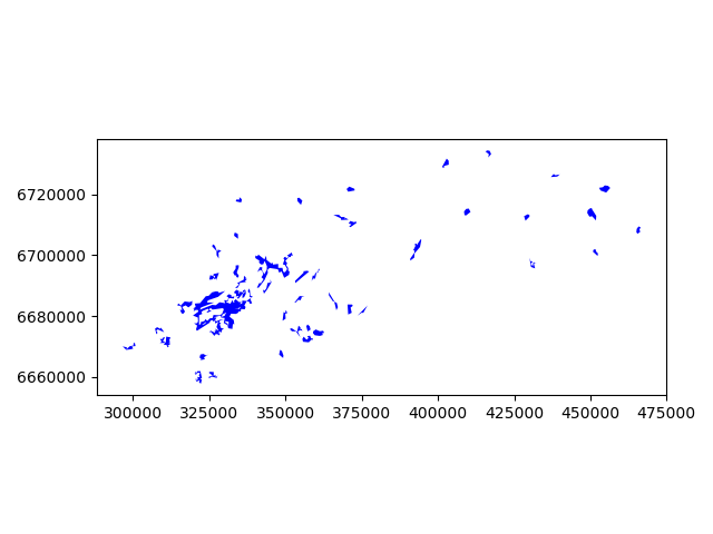
- Let’s see how they look
In [17]: big_lakes.plot(linewidth=0.05, color='blue');

In [18]: plt.tight_layout()

The Polygons that are presented there are quite detailed, let’s generalize them a bit.
- Generalization can be done easily by using a Shapely function called
.simplify(). Thetoleranceparameter is adjusts how much
geometries should be generalized. The tolerance value is tied to the coordinate system of the geometries. Thus, here the value we pass is 300 meters.
In [19]: big_lakes['geom_gen'] = big_lakes.simplify(tolerance=300)
- Let’s set the geometry to be our new column, and plot the results.
In [20]: big_lakes['geometry'] = big_lakes['geom_gen']

In [21]: big_lakes.plot(linewidth=0.05, color='blue')
Out[21]: <matplotlib.axes._subplots.AxesSubplot at 0x2ce1ce29da0>

In [22]: plt.tight_layout()

Nice! As a result, now we have simplified our Polygons slightly (although the differences might be a bit hard to spot).