Network analysis in Python
Finding a shortest path using a specific street network is a common GIS problem that has many practical applications. For example navigators are one of those “every-day” applications where routing using specific algorithms is used to find the optimal route between two (or multiple) points.
It is also possible to perform network analysis such as tranposrtation routing in Python. Networkx is a Python module that provides a lot tools that can be used to analyze networks on various different ways. It also contains algorithms such as Dijkstras algorithm or A* algoritm that are commonly used to find shortest paths along transportation network.
To be able to conduct network analysis, it is, of course, necessary to have a network that is used for the analyses.
Osmnx package that we just explored in previous tutorial, makes it really easy to
retrieve routable networks from OpenStreetMap with different transport modes (walking, cycling and driving). Osmnx also
combines some functionalities from networkx module to make it straightforward to conduct routing along OpenStreetMap data.
Next we will test the routing functionalities of osmnx by finding a shortest path between two points based on drivable roads.
Let’s first download the OSM data from Kamppi but this time include only such street segments that are walkable.
In omsnx it is possible to retrieve only such streets that are drivable by specifying 'drive' into network_type parameter that can be used to
specify what kind of streets are retrieved from OpenStreetMap (other possibilities are walk and bike).
In [1]: import osmnx as ox
In [2]: import networkx as nx
In [3]: import geopandas as gpd
In [4]: import matplotlib.pyplot as plt
In [5]: import pandas as pd
In [6]: place_name = "Kamppi, Helsinki, Finland"
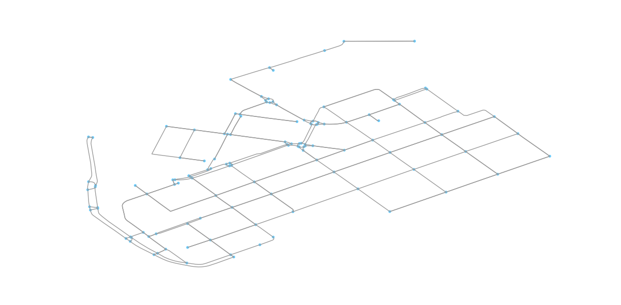
In [7]: graph = ox.graph_from_place(place_name, network_type='drive')
In [8]: fig, ax = ox.plot_graph(graph)
Okey so now we have retrieved only such streets where it is possible to drive with a car. Let’s confirm this by taking a look at the attributes of the street network. Easiest way to do this is to convert the graph (nodes and edges) into GeoDataFrames.
In [9]: edges = ox.graph_to_gdfs(graph, nodes=False, edges=True)
- Let’s check what columns do we have in our data
In [10]: edges.columns
Out[10]:
Index(['bridge', 'geometry', 'highway', 'key', 'lanes', 'length', 'maxspeed',
       'name', 'oneway', 'osmid', 'u', 'v'],
      dtype='object')
Okey, so we have quite many columns in our GeoDataFrame. Most of the columns are fairly self-exploratory but the following table describes all of them.
| Column | Description | Data type |
|---|---|---|
| bridge | Bridge feature | boolean |
| geometry | Geometry of the feature | Shapely.geometry |
| highway | Tag for roads, paths (road type) | str (list if multiple) |
| lanes | Number of lanes | int (or nan) |
| lenght | The length of a feature in meters | float |
| maxspeed | maximum legal speed limit | int (list if multiple) |
| name | Name of the (street) element | str (or nan) |
| oneway | Street is usable only in one direction | boolean |
| osmid | Unique node ids of the element | list |
| u | The first node of networkx edge tuple | int |
| v | The last node of networkx edge tuple | int |
Most of the attributes comes directly from the OpenStreetMap, however, columns u and v are networkx specific ids.
- Let’s take a look what kind of features we have in
highwaycolumn.
In [11]: edges['highway'].value_counts()
Out[11]:
residential 110
tertiary 82
primary 25
secondary 18
unclassified 11
living_street 4
primary_link 1
Name: highway, dtype: int64
In [12]: print("Coordinate system:", edges.crs)
�����������������������������������������������������������������������������������������������������������������������������������������������������������������������������������������Coordinate system: {'init': 'epsg:4326'}
Okey, now we can confirm that as a result our street network indeed only contains such streets where it is allowed to drive with a car as there are no e.g. cycleways of footways included in the data. We can also see that the CRS of the GeoDataFrame seems to be WGS84 (i.e. epsg: 4326).
Let’s continue and find the shortest path between two points based on the distance. As the data is in WGS84 format, we might first want to reproject our data into metric system so that our map looks better.
Luckily there is a handy function in osmnx called project_graph() to project the graph data in UTM format.
In [13]: graph_proj = ox.project_graph(graph)

In [14]: fig, ax = ox.plot_graph(graph_proj)

In [15]: plt.tight_layout()
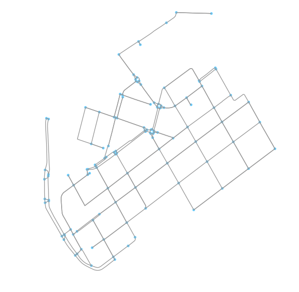
- Let’s see how our data looks like now.
In [16]: nodes_proj, edges_proj = ox.graph_to_gdfs(graph_proj, nodes=True, edges=True)
In [17]: print("Coordinate system:", edges_proj.crs)
Coordinate system: {'datum': 'NAD83', 'ellps': 'GRS80', 'proj': 'utm', 'zone': 35, 'units': 'm'}
In [18]: edges_proj.head()
�������������������������������������������������������������������������������������������������Out[18]:
bridge geometry highway key \
0 NaN LINESTRING (384627.5455369067 6671580.41232014... primary 0
1 NaN LINESTRING (384626.0520768312 6671454.14883848... primary 0
2 NaN LINESTRING (384644.4188576039 6671561.40362007... primary 0
3 NaN LINESTRING (384644.4188576039 6671561.40362007... primary 0
4 NaN LINESTRING (385515.6177346901 6671500.06500373... tertiary 0
lanes length maxspeed name oneway \
0 2 40.546678 40 Mechelininkatu True
1 2 16.621387 40 Mechelininkatu True
2 2 29.174418 40 NaN True
3 2 242.269892 40 Mechelininkatu True
4 NaN 139.185362 [30, 40] Fredrikinkatu True
osmid u v
0 [23856784, 31503767] 25216594 1372425714
1 [29977177, 30470347] 25238874 1372425713
2 [372440330, 8135861] 25238944 25216594
3 [25514547, 30288797, 30288799] 25238944 319896278
4 [30568275, 36729015, 316590744, 316590745, 316... 25291537 25291591
Okey, as we can see from the CRS the data is now in UTM projection using zone 35 which is the one used for Finland, and indeed the orientation of the map and the geometry values also confirm this.
Analyzing the network properties
Now as we have seen some of the basic functionalities of osmnx such as downloading the data and converting data from graph to GeoDataFrame, we can take a look some of the analytical features of omsnx. Osmnx includes many useful functionalities to extract information about the network.
- To calculate some of the basic street network measures we can use
basic_stats()function of osmnx
In [19]: stats = ox.basic_stats(graph_proj)

In [20]: stats
Out[20]:
{'circuity_avg': 1.2765042570918806e-05,
 'clean_intersection_count': None,
 'clean_intersection_density_km': None,
 'edge_density_km': None,
 'edge_length_avg': 78.835341593345689,
 'edge_length_total': 19787.670739929767,
 'intersection_count': 115,
 'intersection_density_km': None,
 'k_avg': 4.08130081300813,
 'm': 251,
 'n': 123,
 'node_density_km': None,
 'self_loop_proportion': 0.0,
 'street_density_km': None,
 'street_length_avg': 75.031938093148469,
 'street_length_total': 13505.748856766724,
 'street_segments_count': 180,
 'streets_per_node_avg': 3.1951219512195124,
 'streets_per_node_counts': {0: 0, 1: 8, 2: 1, 3: 73, 4: 41},
 'streets_per_node_proportion': {0: 0.0,
  1: 0.06504065040650407,
  2: 0.008130081300813009,
  3: 0.5934959349593496,
  4: 0.3333333333333333}}
To be able to extract the more advanced statistics (and some of the missing ones above) from the street network, it is required to have information about the coverage area of the network. Let’s calculate the area of the convex hull of the street network and see what we can get. As certain statistics are produced separately for each node, they produce a lot of output. Let’s merge both stats and put them into Pandas Series to keep things mroe compact.
In [21]: area = edges_proj.unary_union.convex_hull.area

In [22]: stats = ox.basic_stats(graph_proj, area=area)

In [23]: extended_stats = ox.extended_stats(graph_proj, ecc=True, bc=True, cc=True)

In [24]: for key, value in extended_stats.items():
   ....:     stats[key] = value
   ....:

In [25]: pd.Series(stats)
Out[25]:
avg_neighbor_degree                    {25216594: 2.0, 25238874: 2.0, 25238944: 1.0, ...
avg_neighbor_degree_avg                                                          2.16599
avg_weighted_neighbor_degree           {25216594: 0.04932586528128221, 25238874: 0.12...
avg_weighted_neighbor_degree_avg                                               0.0773233
betweenness_centrality                 {25216594: 0.03962877658853814, 25238874: 0.06...
betweenness_centrality_avg                                                     0.0679948
center                                                                      [1372376937]
circuity_avg                                                                  1.2765e-05
clean_intersection_count                                                            None
clean_intersection_density_km                                                       None
closeness_centrality                   {25216594: 0.000856552987043, 25238874: 0.0009...
closeness_centrality_avg                                                      0.00141561
clustering_coefficient                 {25216594: 0, 25238874: 0, 25238944: 0, 252915...
clustering_coefficient_avg                                                     0.0867209
clustering_coefficient_weighted        {25216594: 0, 25238874: 0, 25238944: 0, 252915...
clustering_coefficient_weighted_avg                                            0.0157325
degree_centrality                      {25216594: 0.02459016393442623, 25238874: 0.02...
degree_centrality_avg                                                          0.0334533
diameter                                                                         2139.02
eccentricity                           {25216594: 1900.88375336, 25238874: 1774.60317...
edge_density_km                                                                  24654.7
edge_length_avg                                                                  78.8353
edge_length_total                                                                19787.7
intersection_count                                                                   115
intersection_density_km                                                          143.286
k_avg                                                                             4.0813
m                                                                                    251
n                                                                                    123
node_density_km                                                                  153.253
pagerank                               {25216594: 0.00906630275862, 25238874: 0.00840...
pagerank_max                                                                   0.0242956
pagerank_max_node                                                               25416262
pagerank_min                                                                  0.00140976
pagerank_min_node                                                             1861896879
periphery                                                                    [319896278]
radius                                                                           993.275
self_loop_proportion                                                                   0
street_density_km                                                                16827.7
street_length_avg                                                                75.0319
street_length_total                                                              13505.7
street_segments_count                                                                180
streets_per_node_avg                                                             3.19512
streets_per_node_counts                                 {0: 0, 1: 8, 2: 1, 3: 73, 4: 41}
streets_per_node_proportion            {0: 0.0, 1: 0.06504065040650407, 2: 0.00813008...
dtype: object
Okey, now we have a LOT of information about our street network that can be used to understand its structure.
We can for example see that the average node density in our network is 153 nodes/km and that the total edge length of our network is 19787.7 meters.
Furthermore, we can see that the degree centrality of our network is
on average 0.0334533. Degree is a simple centrality measure that counts how many neighbors a node has (here a fraction of nodes it is connected to).
Another interesting measure is the PageRank that measures the importance of specific node
in the graph. Here we can see that the most important node in our graph seem to a node with osmid 25416262.
PageRank was the algorithm that Google first developed (Larry Page & Sergei Brin) to order the search engine results and became famous for.
You can read the Wikipedia article about different centrality measures if you are interested what the other centrality measures mean.
Hint
There are a lot of good examples of different ways to analyze the network properties with osmnx. Take a look at the Osmnx examples repository.
Shortest path analysis
Let’s now calculate the shortest path between two points. First we need to specify the source and target locations for our route. Let’s use the centroid of our network as the source location and the furthest point in East in our network as the target location.
Let’s first determine the centroid of our network. We can take advantage of the bounds attribute to find out the bounding boxes for each feature in our data. We then make a unary union of those features and make a bounding box geometry out of those values that enables us to determine the centroid of our data.
- This is what the bounds command gives us.
In [26]: edges_proj.bounds.head()
Out[26]:
            minx          miny           maxx          maxy
0  384624.169951  6.671540e+06  384627.545537  6.671580e+06
1  384626.052077  6.671438e+06  384627.546229  6.671454e+06
2  384627.545537  6.671561e+06  384644.418858  6.671580e+06
3  384639.622763  6.671561e+06  384649.706783  6.671803e+06
4  385439.278555  6.671500e+06  385515.617735  6.671617e+06
Okey so it is a DataFrame of minimum and maximum x- and y coordinates.
- Let’s create a bounding box out of those.
In [27]: from shapely.geometry import box

In [28]: bbox = box(*edges_proj.unary_union.bounds)

In [29]: print(bbox)
POLYGON ((385779.4656930579 6671142.734205207, 385779.4656930579 6672267.056878939, 384624.1699512366 6672267.056878939, 384624.1699512366 6671142.734205207, 385779.4656930579 6671142.734205207))
Okey so as a result we seem to have a Polygon, but what actually happened here? First of all, we took the Geometries from our edges_proj GeoDataFrame (123 features) and made a unary union of those features (as a result we have a MultiLineString).
From the MultiLineString we can retrieve the maximum and minimum x and y coordinates of the geometry using the bounds attribute.
The bounds command returns a tuple of four coordinates (minx, miny, maxx, maxy). As a final step we feed those coordinates into box() function that creates a shapely.Polygon object out of those coordinates.
The * -character is used to unpack the values from the tuple (see details)
- Now we can extract the centroid of our bounding box as the source location.
In [30]: orig_point = bbox.centroid

In [31]: print(orig_point)
POINT (385201.8178221472 6671704.895542073)
- Let’s now find the easternmost node in our street network. We can do this by calculating the x coordinates and finding out which node has the largest x-coordinate value. Let’s ensure that the values are floats.
In [32]: nodes_proj['x'] = nodes_proj.x.astype(float)

In [33]: maxx = nodes_proj['x'].max()
- Let’s retrieve the target Point having the largest x-coordinate. We can do this by using the .loc function of Pandas that we have used already many times in earlier tutorials.
In [34]: target_loc = nodes_proj.loc[nodes_proj['x']==maxx, :]

In [35]: print(target_loc)
         highway      lat      lon     osmid              x            y  \
25291564     NaN  60.1659  24.9417  25291564  385779.465693  6.67167e+06

                                             geometry
25291564  POINT (385779.4656930579 6671672.812631538)
Okey now we can see that as a result we have a GeoDataFrame with only one node and the information associated with it.
- Let’s extract the Point geometry from the data.
In [36]: target_point = target_loc.geometry.values[0]

In [37]: print(target_point)
POINT (385779.4656930579 6671672.812631538)
- Let’s now find the nearest graph nodes (and their node-ids) to these points. For osmnx we need to parse the coordinates of the Point as coordinate-tuple with Latitude, Longitude coordinates.
As our data is now projected to UTM projection, we need to specify with method parameter that the function uses
‘euclidean’ distances to calculate the distance from the point to the closest node.
This becomes important if you want to know the actual distance between the Point and the closest node which you can retrieve by specifying parameter return_dist=True.
In [38]: orig_xy = (orig_point.y, orig_point.x)
In [39]: target_xy = (target_point.y, target_point.x)
In [40]: orig_node = ox.get_nearest_node(graph_proj, orig_xy, method='euclidean')
In [41]: target_node = ox.get_nearest_node(graph_proj, target_xy, method='euclidean')
In [42]: o_closest = nodes_proj.loc[orig_node]
In [43]: t_closest = nodes_proj.loc[target_node]
In [44]: print(orig_node)
1372441183
In [45]: print(target_node)
�����������25291564
- Let’s make a GeoDataFrame out of these series
In [46]: od_nodes = gpd.GeoDataFrame([o_closest, t_closest], geometry='geometry', crs=nodes_proj.crs)
Okey, as a result we got now the closest node-ids of our origin and target locations.
- Now we are ready to do the routing and find the shortest path between the origin and target locations
by using the shortest_path() function of networkx.
With weight -parameter we can specify that 'length' attribute should be used as the cost impedance in the routing.
In [47]: route = nx.shortest_path(G=graph_proj, source=orig_node, target=target_node, weight='length')

In [48]: print(route)
[1372441183, 1372441170, 60170471, 1377211668, 1377211666, 25291565, 25291564]
Okey, as a result we get a list of all the nodes that are along the shortest path. We could extract the locations of those nodes from the nodes_proj GeoDataFrame and create a LineString presentation of the points,
but luckily, osmnx can do that for us and we can plot shortest path by using plot_graph_route() function.
In [49]: fig, ax = ox.plot_graph_route(graph_proj, route, origin_point=orig_xy, destination_point=target_xy)

In [50]: plt.tight_layout()
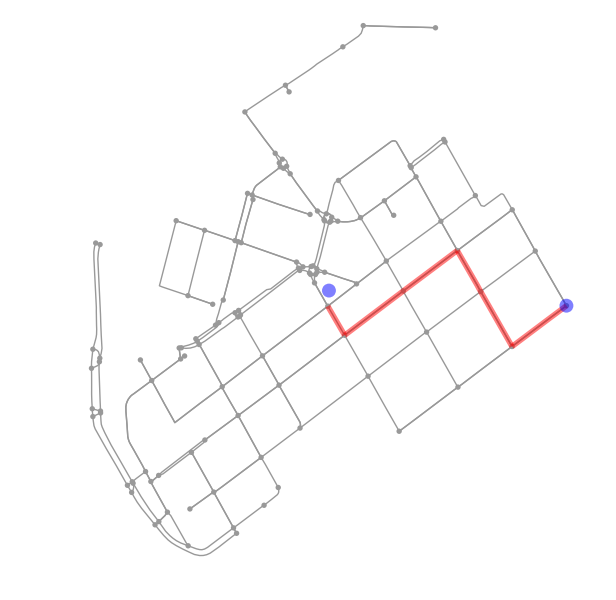
Awesome! Now we have a the shortest path between our origin and target locations. Being able to analyze shortest paths between locations can be valuable information for many applications. Here, we only analyzed the shortest paths based on distance but quite often it is more useful to find the optimal routes between locations based on the travelled time. Here, for example we could calculate the time that it takes to cross each road segment by dividing the length of the road segment with the speed limit and calculate the optimal routes by taking into account the speed limits as well that might alter the result especially on longer trips than here.
Saving shortest paths to disk
Quite often you need to save the route e.g. as a Shapefile. Hence, let’s continue still a bit and see how we can make a Shapefile of our route with some information associated with it.
- First we need to get the nodes that belong to the shortest path.
In [51]: route_nodes = nodes_proj.loc[route]

In [52]: print(route_nodes)
                    highway      lat      lon       osmid              x  \
1372441183              NaN  60.1658  24.9312  1372441183  385199.040421
1372441170              NaN  60.1652   24.932  1372441170  385239.956997
60170471                NaN  60.1661  24.9345    60170471  385382.590390
1377211668              NaN  60.1669  24.9368  1377211668  385514.080701
1377211666              NaN  60.1662  24.9379  1377211666  385570.886276
25291565    traffic_signals  60.1651  24.9393    25291565  385647.135652
25291564                NaN  60.1659  24.9417    25291564  385779.465693

                      y                                     geometry
1372441183  6.67167e+06  POINT (385199.0404211304 6671671.819689871)
1372441170  6.67161e+06  POINT (385239.9569968735 6671610.079883121)
60170471     6.6717e+06  POINT (385382.5903898547 6671704.041333381)
1377211668  6.67179e+06   POINT (385514.080700958 6671789.786299309)
1377211666   6.6717e+06  POINT (385570.8862759892 6671702.891562204)
25291565    6.67159e+06  POINT (385647.1356519004 6671586.226356798)
25291564    6.67167e+06  POINT (385779.4656930579 6671672.812631538)
- Now we can create a LineString out of the Point geometries of the nodes
In [53]: from shapely.geometry import LineString, Point

In [54]: route_line = LineString(list(route_nodes.geometry.values))

In [55]: print(route_line)
LINESTRING (385199.0404211304 6671671.819689871, 385239.9569968735 6671610.079883121, 385382.5903898547 6671704.041333381, 385514.080700958 6671789.786299309, 385570.8862759892 6671702.891562204, 385647.1356519004 6671586.226356798, 385779.4656930579 6671672.812631538)
- Let’s make a GeoDataFrame having some useful information about our route such as a list of the osmids that are part of the route and the length of the route.
In [56]: route_geom = gpd.GeoDataFrame(crs=edges_proj.crs)

In [57]: route_geom['geometry'] = None

In [58]: route_geom['osmids'] = None
- Let’s add the information: geometry, a list of osmids and the length of the route.
In [59]: route_geom.loc[0, 'geometry'] = route_line

In [60]: route_geom.loc[0, 'osmids'] = str(list(route_nodes['osmid'].values))

In [61]: route_geom['length_m'] = route_geom.length
Now we have a GeoDataFrame that we can save to disk. Let’s still confirm that everything is okey by plotting our route on top of our street network, and plot also the origin and target points on top of our map.
- Let’s first prepare a GeoDataFrame for our origin and target points.
In [62]: od_points = gpd.GeoDataFrame(crs=edges_proj.crs)

In [63]: od_points['geometry'] = None

In [64]: od_points['type'] = None

In [65]: od_points.loc[0, ['geometry', 'type']] = orig_point, 'Origin'

In [66]: od_points.loc[1, ['geometry', 'type']] = target_point, 'Target'

In [67]: od_points.head()
Out[67]:
                                      geometry    type
0  POINT (385201.8178221472 6671704.895542073)  Origin
1  POINT (385779.4656930579 6671672.812631538)  Target
- Let’s also get the buildings for our area and plot them as well.
In [68]: buildings = ox.buildings_from_place(place_name)

In [69]: buildings_proj = buildings.to_crs(crs=edges_proj.crs)
- Let’s now plot the route and the street network elements to verify that everything is as it should.
In [70]: fig, ax = plt.subplots()
In [71]: edges_proj.plot(ax=ax, linewidth=0.75, color='gray')
��������������������������������������������������������������������������������������������������������������������������������������������������������������������������������������������������������������������������������������������������������������������������������������������������������������������������������������������������������������������������������������������������������������������������������������������������������������������������������������������������������������������������������������������������������������������������������������������������������������������������������������������������������������������������������������������������������������������������������������������������������������������������������������������������������������������������������������������������������������Out[71]: <matplotlib.axes._subplots.AxesSubplot at 0x2ce1cdb5b38>
In [72]: nodes_proj.plot(ax=ax, markersize=2, color='gray')
��������������������������������������������������������������������������������������������������������������������������������������������������������������������������������������������������������������������������������������������������������������������������������������������������������������������������������������������������������������������������������������������������������������������������������������������������������������������������������������������������������������������������������������������������������������������������������������������������������������������������������������������������������������������������������������������������������������������������������������������������������������������������������������������������������������������������������������������������������������������������������������������������������������������������������Out[72]: <matplotlib.axes._subplots.AxesSubplot at 0x2ce1cdb5b38>
In [73]: buildings_proj.plot(ax=ax, facecolor='khaki', alpha=0.7)
��������������������������������������������������������������������������������������������������������������������������������������������������������������������������������������������������������������������������������������������������������������������������������������������������������������������������������������������������������������������������������������������������������������������������������������������������������������������������������������������������������������������������������������������������������������������������������������������������������������������������������������������������������������������������������������������������������������������������������������������������������������������������������������������������������������������������������������������������������������������������������������������������������������������������������������������������������������������������������������������������Out[73]: <matplotlib.axes._subplots.AxesSubplot at 0x2ce1cdb5b38>
In [74]: route_geom.plot(ax=ax, linewidth=4, linestyle='--', color='red')
��������������������������������������������������������������������������������������������������������������������������������������������������������������������������������������������������������������������������������������������������������������������������������������������������������������������������������������������������������������������������������������������������������������������������������������������������������������������������������������������������������������������������������������������������������������������������������������������������������������������������������������������������������������������������������������������������������������������������������������������������������������������������������������������������������������������������������������������������������������������������������������������������������������������������������������������������������������������������������������������������������������������������������������������������������������������Out[74]: <matplotlib.axes._subplots.AxesSubplot at 0x2ce1cdb5b38>
In [75]: od_points.plot(ax=ax, markersize=24, color='green')
��������������������������������������������������������������������������������������������������������������������������������������������������������������������������������������������������������������������������������������������������������������������������������������������������������������������������������������������������������������������������������������������������������������������������������������������������������������������������������������������������������������������������������������������������������������������������������������������������������������������������������������������������������������������������������������������������������������������������������������������������������������������������������������������������������������������������������������������������������������������������������������������������������������������������������������������������������������������������������������������������������������������������������������������������������������������������������������������������������������������������������������Out[75]: <matplotlib.axes._subplots.AxesSubplot at 0x2ce1cdb5b38>
In [76]: plt.tight_layout()
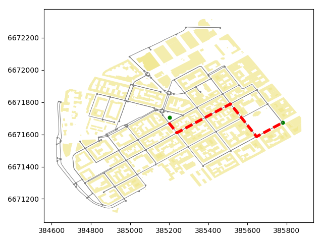
Great everything seems to be in order! As you can see, now we have a full control of all the elements of our map and we can use all the aesthetic properties that matplotlib provides to modify how our map will look like. Now we can save to disk all the elements that we want.
# Parse the place name for the output file names (replace spaces with underscores and remove commas)
In [77]: place_name_out = place_name.replace(' ', '_').replace(',','')

In [78]: streets_out = r"/home/geo/%s_streets.shp" % place_name_out

In [79]: route_out = r"/home/geo/Route_from_a_to_b_at_%s.shp" % place_name_out

In [80]: nodes_out = r"/home/geo/%s_nodes.shp" % place_name_out

In [81]: buildings_out = r"/home/geo/%s_buildings.shp" % place_name_out

In [82]: od_out = r"/home/geo/%s_route_OD_points.shp" % place_name_out
As there are certain columns with such data values that Shapefile format does not support (such as list or boolean), we need to convert those into strings to be able to export the data to Shapefile.
- Columns with invalid values
In [83]: invalid_cols = ['lanes', 'maxspeed', 'name', 'oneway', 'osmid']
- Iterate over invalid columns and convert them to string format
In [84]: for col in invalid_cols:
   ....:     edges_proj[col] = edges_proj[col].astype(str)
   ....:
- Save the data
In [85]: edges_proj.to_file(streets_out)

In [86]: route_geom.to_file(route_out)

In [87]: nodes_proj.to_file(nodes_out)

In [88]: od_points.to_file(od_out)

In [89]: buildings[['geometry', 'name', 'addr:street']].to_file(buildings_out)
Great now we have saved all the data that was used to produce the maps as Shapefiles.