This page was generated from source/notebooks/L4/Point-in-polygon.ipynb.

Point in Polygon & Intersect¶

Finding out if a certain point is located inside or outside of an area, or finding out if a line intersects with another line or polygon are fundamental geospatial operations that are often used e.g. to select data based on location. Such spatial queries are one of the typical first steps of the workflow when doing spatial analysis. Performing a spatial join (will be introduced later) between two spatial datasets is one of the most typical applications where Point in Polygon (PIP) query is used.

Download data¶

For the lesson four download data package from here.

The data package contains a KML-file called PKS_suuralue.kml, addresses.shp, and Vaestotietoruudukko_2015.shp.

How to check if point is inside a polygon?¶

Computationally, detecting if a point is inside a polygon is most commonly done using a specific formula called Ray Casting algorithm. Luckily, we do not need to create such a function ourselves for conducting the Point in Polygon (PIP) query. Instead, we can take advantage of Shapely’s binary predicates that can evaluate the topolocical relationships between geographical objects, such as the PIP as we’re interested here.

There are basically two ways of conducting PIP in Shapely:

using a function called .within() that checks if a point is within a polygon
using a function called .contains()_ that checks if a polygon contains a point

Notice: even though we are talking here about Point in Polygon operation, it is also possible to check if a LineString or Polygon is inside another Polygon.

Let’s first create a Polygon using a list of coordinate-tuples and a couple of Point objects

In [1]:

from shapely.geometry import Point, Polygon

# Create Point objects
p1 = Point(24.952242, 60.1696017)
p2 = Point(24.976567, 60.1612500)

# Create a Polygon
coords = [(24.950899, 60.169158), (24.953492, 60.169158), (24.953510, 60.170104), (24.950958, 60.169990)]
poly = Polygon(coords)

# Let's check what we have
print(p1)
print(p2)
print(poly)

POINT (24.952242 60.1696017)
POINT (24.976567 60.16125)
POLYGON ((24.950899 60.169158, 24.953492 60.169158, 24.95351 60.170104, 24.950958 60.16999, 24.950899 60.169158))

Let’s check if those points are within the polygon

In [2]:

# Check if p1 is within the polygon using the within function
p1.within(poly)

# Check if p2 is within the polygon
p2.within(poly)

Out[2]:

False

Okey, so we can see that the first point seems to be inside that polygon and the other one doesn’t.

In fact, the first point is close to the center of the polygon as we can see:

In [4]:

# Our point
print(p1)

# The centroid
print(poly.centroid)

POINT (24.952242 60.1696017)
POINT (24.95224242849236 60.16960179038188)

It is also possible to do PIP other way around, i.e. to check if polygon contains a point:

In [6]:

# Does polygon contain p1?
poly.contains(p1)

# Does polygon contain p2?
poly.contains(p2)

Out[6]:

False

Thus, both ways of checking the spatial relationship results in the same way.

Which one should you use then? Well, it depends:

if you have many points and just one polygon and you try to find out which one of them is inside the polygon:
- you need to iterate over the points and check one at a time if it is within() the polygon specified
if you have many polygons and just one point and you want to find out which polygon contains the point
- you need to iterate over the polygons until you find a polygon that contains() the point specified (assuming there are no overlapping polygons)

Intersect¶

Another typical geospatial operation is to see if a geometry intersect or touches another one. The difference between these two is that:

if objects intersect, the boundary and interior of an object needs to intersect in any way with those of the other.
If an object touches the other one, it is only necessary to have (at least) a single point of their boundaries in common but their interiors shoud NOT intersect.

Let’s try these out.

Let’s create two LineStrings

In [7]:

from shapely.geometry import LineString, MultiLineString

# Create two lines
line_a = LineString([(0, 0), (1, 1)])
line_b = LineString([(1, 1), (0, 2)])

Let’s see if they intersect

In [8]:

line_a.intersects(line_b)

Out[8]:

True

Do they also touch each other?

In [9]:

line_a.touches(line_b)

Out[9]:

True

Indeed, they do and we can see this by plotting the features together

In [10]:

# Create a MultiLineString
multi_line = MultiLineString([line_a, line_b])
multi_line

Out[10]:

../../_images/notebooks_L4_Point-in-polygon_15_0.svg

Thus, the line_b continues from the same node ( (1,1) ) where line_a ends.

However, if the lines overlap fully, they don’t touch due to the spatial relationship rule, as we can see:

Check if line_a touches itself

In [11]:

# Does the line touch with itself?
line_a.touches(line_a)

Out[11]:

False

It does not. However, it does intersect

In [12]:

# Does the line intersect with itself?
line_a.intersects(line_a)

Out[12]:

True

Point in Polygon using Geopandas¶

Next we will do a practical example where we check which of the addresses from previous tutorial are located in Southern district of Helsinki. We will use a KML-file that has the Polygons for districts of Helsinki Region (data openly available from Helsinki Region Infoshare.

Let’s start by reading the addresses from the Shapefile that we saved earlier.

In [3]:

import geopandas as gpd
fp = "L4_data/addresses.shp"
data = gpd.read_file(fp)

Reading KML-files in Geopandas¶

It is possible to read the data from KML-file in a similar manner as Shapefile. However, we need to first, enable the KML-driver which is not enabled by default (because KML-files can contain unsupported data structures, nested folders etc., hence be careful when reading KML-files).

Let’s enable the read and write functionalities for KML-driver by passing 'rw' to whitelist of fiona’s supported drivers:

In [5]:

import geopandas as gpd
import matplotlib.pyplot as plt
gpd.io.file.fiona.drvsupport.supported_drivers['KML'] = 'rw'

Now we should be able to read a KML file with Geopandas.

Let’s read the data from a following KML -file:

In [6]:

# Filepath to KML file
fp = "L4_data/PKS_suuralue.kml"

polys = gpd.read_file(fp, driver='KML')
polys

Out[6]:

	Name	geometry
0	Suur-Espoonlahti	POLYGON Z ((24.775059677807 60.1090604462157 0...
1	Suur-Kauklahti	POLYGON Z ((24.6157775254076 60.1725681273527 ...
2	Vanha-Espoo	POLYGON Z ((24.6757633262026 60.2120070032819 ...
3	Pohjois-Espoo	POLYGON Z ((24.767921197401 60.2691954732391 0...
4	Suur-Matinkylä	POLYGON Z ((24.7536131356802 60.1663051341717 ...
5	Kauniainen	POLYGON Z ((24.6907528033566 60.2195779731868 ...
6	Suur-Leppävaara	POLYGON Z ((24.797472695835 60.2082651196077 0...
7	Suur-Tapiola	POLYGON Z ((24.8443596422129 60.1659790707387 ...
8	Myyrmäki	POLYGON Z ((24.8245867448802 60.2902531157585 ...
9	Kivistö	POLYGON Z ((24.9430919106369 60.3384471629062 ...
10	Eteläinen	POLYGON Z ((24.7827651307035 60.09997268858 0,...
11	Kaakkoinen	POLYGON Z ((24.8480782099727 60.0275589731893 ...
12	Keskinen	POLYGON Z ((24.9085548098731 60.2082029641503 ...
13	Läntinen	POLYGON Z ((24.832174555671 60.2516121985945 0...
14	Pohjoinen	POLYGON Z ((24.8992644865152 60.2689368800439 ...
15	Koillinen	POLYGON Z ((24.9722813313308 60.2432476462193 ...
16	Aviapolis	POLYGON Z ((24.9430919106369 60.3384471629062 ...
17	Tikkurila	POLYGON Z ((24.9764047156358 60.2896890295612 ...
18	Koivukylä	POLYGON Z ((24.9942315864552 60.3329637072809 ...
19	Itäinen	POLYGON Z ((25.0351655840904 60.23627484214 0,...
20	Östersundom	POLYGON Z ((25.233518559787 60.2565486562817 0...
21	Hakunila	POLYGON Z ((25.0847165922124 60.2724847557756 ...
22	Korso	POLYGON Z ((25.1238010972777 60.341907177167 0...

Nice, now we can see that we have 22 districts in our area. We are interested in an area that is called Eteläinen (‘Southern’ in english).

Let’s select that one and see where it is located, and plot also the points on top of the map.

In [8]:

%matplotlib inline
import matplotlib.pyplot as plt

# Select 'Eteläinen' district (Southern)
southern = polys.loc[polys['Name']=='Eteläinen']
southern.reset_index(drop=True, inplace=True)

# Create plot
ax = polys.plot(facecolor='gray');
southern.plot(ax=ax, facecolor='red');
data.plot(ax=ax, color='blue', markersize=5);
plt.tight_layout()

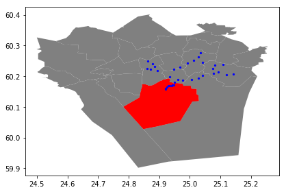
../../_images/notebooks_L4_Point-in-polygon_27_0.png

Okey, so we can see that, indeed, certain points are within the selected red Polygon.

Let’s find out which one of them are located within the Polygon. Hence, we are conducting a Point in Polygon query.

Let’s first enable shapely.speedups which makes some of the spatial queries running faster.

In [9]:

import shapely.speedups
shapely.speedups.enable()

Let’s check which Points are within the southern Polygon. Notice, that here we check if the Points are within the geometry of the southern GeoDataFrame. Hence, we use the loc[0, 'geometry'] to parse the actual Polygon geometry object from the GeoDataFrame.

In [11]:

# Create a mask
pip_mask = data.within(southern.loc[0, 'geometry'])
print(pip_mask)

0      True
1      True
2     False
3     False
4      True
5     False
6     False
7     False
8     False
9     False
10     True
11    False
12    False
13    False
14    False
15    False
16    False
17    False
18    False
19    False
20    False
21    False
22    False
23    False
24    False
25    False
26    False
27    False
28    False
29    False
30     True
31     True
32     True
33     True
34    False
dtype: bool

As we can see, we now have an array of boolean values for each row, where the result is True if Point was inside the Polygon, and False if it was not.

We can now use this mask array to select the Points that are inside the Polygon. Selecting data with this kind of mask array (of boolean values) is easy by passing the array inside the loc indexing function of Pandas.

In [12]:

# Select points that are within Polygon
pip_data = data.loc[pip_mask]
pip_data

Out[12]:

	address	id	geometry
0	Kampinkuja 1, 00100 Helsinki, Finland	1001	POINT (24.9301701 60.1683731)
1	Kaivokatu 8, 00101 Helsinki, Finland	1002	POINT (24.9418933 60.1698665)
4	Tyynenmerenkatu 9, 00220 Helsinki, Finland	1005	POINT (24.9214846 60.1565781)
10	Rautatientori 1, 00100 Helsinki, Finland	1011	POINT (24.94251 60.1711874)
30	Urho Kekkosen katu 1, 00100 Helsinki, Finland	1031	POINT (24.9337569 60.1694809)
31	Gräsviksgatan 17, 00101 Helsingfors, Finland	1032	POINT (24.9250072 60.16500139999999)
32	Stillahavsgatan 3, 00220 Helsingfors, Finland	1033	POINT (24.9214046 60.159069)
33	Vilhelmsgatan 4, 00101 Helsingfors, Finland	1034	POINT (24.9468514 60.1719108)

Let’s finally confirm that our Point in Polygon query worked as it should by plotting the data.

In [17]:

# Plot
ax = polys.plot(facecolor='gray')
southern.plot(ax=ax, facecolor='red')
pip_data.plot(ax=ax, color='gold', markersize=2)
plt.tight_layout()

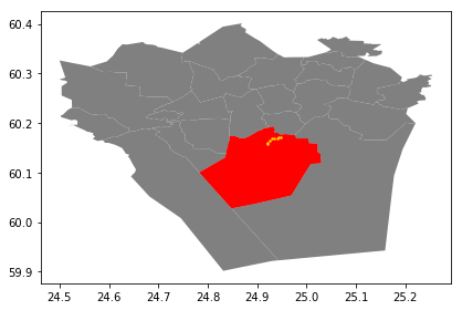
../../_images/notebooks_L4_Point-in-polygon_35_0.png

Perfect! Now we only have the (golden) points that, indeed, are inside the red Polygon which is exactly what we wanted!