This page was generated from source/notebooks/L5/clipping-raster.ipynb.

Masking / clipping raster¶

One common task in raster processing is to clip raster files based on a Polygon. The following example shows how to clip a large raster based on a bounding box around Helsinki Region.

Import modules and specify the input and output filepaths

In [21]:

import rasterio
from rasterio.plot import show
from rasterio.plot import show_hist
from rasterio.mask import mask
from shapely.geometry import box
import geopandas as gpd
from fiona.crs import from_epsg
import pycrs
import os
%matplotlib inline

# Data dir
data_dir = "L5_data"

# Input raster
fp = os.path.join(data_dir, "p188r018_7t20020529_z34__LV-FIN.tif")

# Output raster
out_tif = os.path.join(data_dir, "Helsinki_Masked.tif")

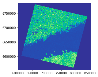
Let’s start by opening the raster in read mode and visualizing it (using specific colormap called terrain):

In [7]:

# Read the data
data = rasterio.open(fp)

# Visualize the NIR band
show((data, 4), cmap='terrain')

../../_images/notebooks_L5_clipping-raster_4_0.png

Out[7]:

<matplotlib.axes._subplots.AxesSubplot at 0x19996e3d7b8>

Okey, as you can see, we have a huge raster file where we can see the coastlines of Finland and Estonia. What we want to do next is to create a bounding box around Helsinki region and clip the raster based on that.

Next, we need to create a bounding box for our area of interest with Shapely.

In [8]:

# WGS84 coordinates
minx, miny = 24.60, 60.00
maxx, maxy = 25.22, 60.35
bbox = box(minx, miny, maxx, maxy)

Create a GeoDataFrame from the bounding box

In [9]:

geo = gpd.GeoDataFrame({'geometry': bbox}, index=[0], crs=from_epsg(4326))
print(geo)

                                            geometry
0  POLYGON ((25.22 60, 25.22 60.35, 24.6 60.35, 2...

As we can see now we have a GeoDataFrame with Polygon inside. To be able to clip the raster with this Polygon, it is required that the data has identical coordinate reference system.

Re-project into the same coordinate system as the raster data. We can access the crs of the raster using attribute .crs.data:

In [11]:

# Project the Polygon into same CRS as the grid
geo = geo.to_crs(crs=data.crs.data)

# Print crs
geo.crs

Out[11]:

{'init': 'epsg:32634'}

Next we need to get the coordinates of the geometry in such a format that rasterio wants them. This can be conducted easily with following function:

In [12]:

def getFeatures(gdf):
    """Function to parse features from GeoDataFrame in such a manner that rasterio wants them"""
    import json
    return [json.loads(gdf.to_json())['features'][0]['geometry']]

Get the geometry coordinates by using the function.

In [13]:

coords = getFeatures(geo)
print(coords)

[{'type': 'Polygon', 'coordinates': [[[735275.3533476053, 6658919.843253607], [732783.55612074, 6697846.086795722], [698608.1329965619, 6695816.080575278], [700733.5832412266, 6656875.248540204], [735275.3533476053, 6658919.843253607]]]}]

Okay, as we can see rasterio wants to have the coordinates of the Polygon in GeoJSON format.

Now we are ready to clip the raster with the polygon using the coords variable that we just created. Clipping the raster can be done easily with the mask function that we imported in the beginning from rasterio, and specifying clip=True.

In [16]:

# Clip the raster with Polygon
out_img, out_transform = mask(dataset=data, shapes=coords, crop=True)

Next, we need to modify the metadata. Let’s start by copying the metadata from the original data file.

In [17]:

# Copy the metadata
out_meta = data.meta.copy()
print(out_meta)

{'driver': 'GTiff', 'dtype': 'uint8', 'nodata': None, 'width': 8877, 'height': 8106, 'count': 7, 'crs': CRS({'init': 'epsg:32634'}), 'transform': Affine(28.5, 0.0, 600466.5,
       0.0, -28.5, 6784966.5)}

Next we need to parse the EPSG value from the CRS so that we can create a Proj4 -string using PyCRS library (to ensure that the projection information is saved correctly).

In [18]:

# Parse EPSG code
epsg_code = int(data.crs.data['init'][5:])
print(epsg_code)

Now we need to update the metadata with new dimensions, transform (affine) and CRS (as Proj4 text):

In [19]:

out_meta.update({"driver": "GTiff",
                 "height": out_img.shape[1],
                 "width": out_img.shape[2],
                 "transform": out_transform,
                 "crs": pycrs.parser.from_epsg_code(epsg_code).to_proj4()}
                         )

Finally, we can save the clipped raster to disk with following command:

In [22]:

with rasterio.open(out_tif, "w", **out_meta) as dest:
        dest.write(out_img)

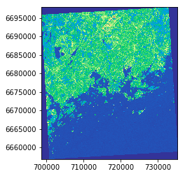
Let’s still check that the result is correct by plotting our new clipped raster.

In [23]:

# Open the clipped raster file
clipped = rasterio.open(out_tif)

# Visualize
show((clipped, 5), cmap='terrain')

../../_images/notebooks_L5_clipping-raster_26_0.png

Out[23]:

<matplotlib.axes._subplots.AxesSubplot at 0x19980263fd0>

Great, it worked! This is how you can easily clip (mask) raster files with rasterio.