Map projections
Coordinate reference systems (CRS) are important because the geometric shapes in a GeoDataFrame are simply a collection of coordinates in an arbitrary space. A CRS tells Python how those coordinates are related to places on the Earth. A map projection (or a projected coordinate system) is a systematic transformation of the latitudes and longitudes into a plain surface where units are quite commonly represented as meters (instead of decimal degrees). This transformation is used to represent the three dimensional earth on a flat, two dimensional map.
As the CRS in different spatial datasets differ fairly often (i.e. one might have coordinates defined in decimal degrees while the other one has them in meters), it is a common procedure to redefine (or reproject) the CRS to be identical in both layers. It is important that the layers have the same coordinate reference system as it makes it possible to analyze the spatial relationships between the layers, such as conduct a Point in Polygon -query.
Choosing an appropriate projection for your map is not always straightforward because it depends on what you actually want to represent with your map, and what is the spatial scale of your data. In fact, there does not exist a “perfect projection” since each one of them has some strengths and weaknesses, and you should choose such projection that fits best for your needs. In fact, the projection you choose might even tell something about you:
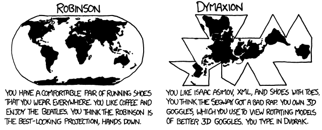 Source: XKCD, See a full comic about“What your favorite
map projection tells about you”.
Source: XKCD, See a full comic about“What your favorite
map projection tells about you”.
For those of you who want a bit more analytical approach for choosing the projection, you can get a good overview from georeference.org, or from this blog post introducing the strengths and weaknesses of a few commonly used projections.
Coordinate reference system (CRS) in Geopandas
Luckily, defining and changing projections is easy in Geopandas. In this tutorial we will see how to retrieve the coordinate reference system information from the data, and how to change it. We will re-project a data file from WGS84 (lat, lon coordinates) into a Lambert Azimuthal Equal Area projection which is the recommended projection for Europe by European Commission.
For this tutorial we will be using a Shapefile called
Europe_borders.shp representing the country borders in Europe, that
you already should have downloaded during the previous
tutorial.
Shapefile should always contain information about the coordinate
reference system that is stored in .prj -file (at least if the data
has been appropriately produced). When reading the data into
GeoDataFrame with Geopandas this information is automatically stored
into .crs attribute of the GeoDataFrame.
- Let’s start by reading the data from the
Europe_borders.shpfile and checking thecrs:
In [1]:
# Import necessary packages
import geopandas as gpd

# Read the file
fp = "L2_data/Europe_borders.shp"
data = gpd.read_file(fp)

# Check the coordinate reference system
data.crs
Out[1]:
{'init': 'epsg:4326'}
As we can see, here, the crs is a Python dictionary with a key
init that has a value epsg:4326. This is a very typical way how
CRS is stored in GeoDataFrames. There is also another typical way of
representing the coordinate reference system, namely storing that
information in
Proj4-string format (we
will come back to this later).
The EPSG number (“European Petroleum Survey Group”) is a code that
tells about the coordinate system of the dataset. “EPSG Geodetic
Parameter Dataset is a collection of
definitions of coordinate reference systems and coordinate
transformations which may be global, regional, national or local in
application”. EPSG code 4326 that we have here, belongs to the WGS84
coordinate system (i.e. coordinates are in decimal degrees: latitudes
and longitudes).
You can find a lot of information and lists of available coordinate reference systems from:
- www.spatialreference.org
- www.proj4.org
- www.mapref.org
- Let’s continue by checking the values in our
geometry-column to verify that the CRS of our GeoDataFrame seems correct:
In [2]:
data['geometry'].head()
Out[2]:
0    POLYGON ((8.457777976989746 54.56236267089844,...
1    POLYGON ((8.71992015838623 47.69664382934571, ...
2    POLYGON ((6.733166694641113 53.5740852355957, ...
3    POLYGON ((6.858222007751465 53.59411239624024,...
4    POLYGON ((6.89894437789917 53.6256103515625, 6...
Name: geometry, dtype: object
As we can see, the coordinate values of the Polygons indeed look like latitude and longitude values, so everything seems to be in order (as in most cases).
WGS84 projection is not really a good one for representing European borders, so let’s convert those geometries into Lambert Azimuthal Equal Area projection (EPSG: 3035) which is the recommended projection by European Comission.
Changing the projection is simple to do in
Geopandas with
.to_crs() -function which is a built-in function of the
GeoDataFrame. The function has two alternative parameters 1) crs and
2) epgs that can be used to make the coordinate transformation and
re-project the data into the CRS that you want to use.
- Let’s re-project our data into
EPSG 3035usingepsg-parameter:
In [3]:
# Let's make a copy of our data
orig = data.copy()

# Reproject the data
data = data.to_crs(epsg=3035)

# Check the new geometry values
print(data['geometry'].head())
0    POLYGON ((4221214.558088431 3496203.404338956,...
1    POLYGON ((4224860.478308966 2732279.319617757,...
2    POLYGON ((4104652.175545862 3390034.953002084,...
3    POLYGON ((4113025.664284974 3391895.755505159,...
4    POLYGON ((4115871.227627173 3395282.099288368,...
Name: geometry, dtype: object
And here we go, the coordinate values in the geometries have changed!
Now we have successfully changed the projection of our layer into a new
one, i.e. to ETRS-LAEA projection.
To really understand what is going on, it is good to explore our data visually. Hence, let’s compare the datasets by making maps out of them.
In [4]:
%matplotlib inline
import matplotlib.pyplot as plt

# Make subplots that are next to each other
fig, (ax1, ax2) = plt.subplots(nrows=1, ncols=2, figsize=(12, 8))

# Plot the data in WGS84 CRS
orig.plot(ax=ax1, facecolor='gray');

# Add title
ax1.set_title("WGS84");

# Plot the one with ETRS-LAEA projection
data.plot(ax=ax2, facecolor='blue');

# Add title
ax2.set_title("ETRS Lambert Azimuthal Equal Area projection");

# Remove empty white space around the plot
plt.tight_layout()
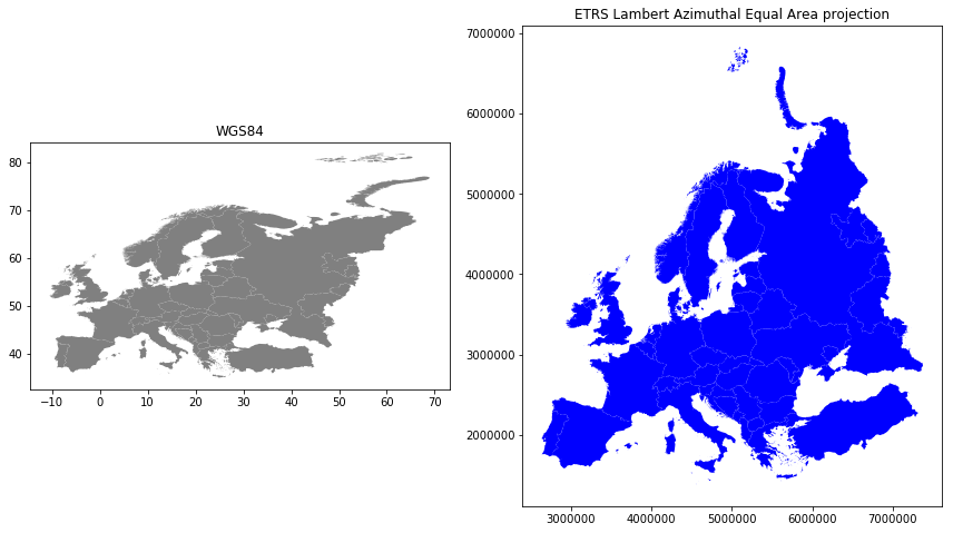
Indeed, the maps look quite different, and the re-projected one looks much better in Europe as the areas especially in the north are more realistic and not so stretched as in WGS84.
- Finally, let’s save our projected layer into a Shapefile so that we can use it later.
In [5]:
# Ouput filepath
outfp = "L2_data/Europe_borders_epsg3035.shp"

# Save to disk
data.to_file(outfp)
NOTICE: On Windows, the .prj -file might NOT update with the
new CRS value when saving to Shapefile. If this happens it is possible
to fix the prj by passing the coordinate reference information as
proj4-string. For this purpose a library called
PyCRS is a handy tool that
makes passing the proj4-strings easy. PyCRS has functions
pycrs.parser.from_epsg_code() and .to_proj4() that can be used
to define the CRS as proj4-string format:
In [6]:
# Import pycrs
import pycrs

# Define the crs for the GeoDataFrame as proj4-string
epsg_code = 3035
data.crs = pycrs.parser.from_epsg_code(epsg_code).to_proj4()

# Let's see what we have now
data.crs
Out[6]:
'+proj=laea +ellps=GRS80 +a=6378137.0 +f=298.257222101 +pm=0 +lon_0=10 +x_0=4321000 +y_0=3210000 +lat_0=52 +units=m +axis=enu +no_defs'
As we can see, now the CRS of the GeoDataFrame is represented as
Proj4-string that will be
saved into the .prj -file when saving the GeoDataFrame into
Shapefile.
- Let’s save the file once more:
In [7]:
# Ouput filepath
outfp = "L2_data/Europe_borders_epsg3035.shp"

# Save to disk
data.to_file(outfp)
The PyCRS library is really useful as it contains information and supports many different coordinate reference definitions, such as OGC WKT (v1), ESRI WKT, Proj4, and any EPSG, ESRI, or SR-ORG code available from spatialreference.org.
Calculating distances
Next, we will conduct a practical example, and continue working with the
Europe_borders.shp -file. Our aim is to find the Euclidean distances
from the centroids (midpoints) of all European countries to Helsinki,
Finland. We will calculate the distance between Helsinki and other
European countries using a metric projection (Azimuthal Equidistant
-projection)
that gives us the distance in meters. Notice, that this projection is
slightly less commonly used, but still useful to know.
- Let’s first create a GeoDataFrame that contains a single Point representing the location of Helsinki, Finland:
In [8]:
# Import necessary modules
from shapely.geometry import Point
import pycrs

# Create the point representing Helsinki (in WGS84)
hki_lon = 24.9417
hki_lat = 60.1666

# Create GeoDataFrame
helsinki = gpd.GeoDataFrame([[Point(hki_lon, hki_lat)]], geometry='geometry', crs={'init': 'epsg:4326'}, columns=['geometry'])

# Print
print(helsinki)
                  geometry
0  POINT (24.9417 60.1666)
As we can see, it is possible to create a GeoDataFrame directly with one
line of code. Notice that, here, we specified the CRS directly by
passing the crs as Python dictionary {'init': 'epsg:4326'} which is
one alternative way to define the CRS. We also told that the
geometry information is stored in column called 'geometry' that
we actually define with parameter columns=['geometry'].
Next, we need to convert this GeoDataFrame to “Azimuthal
Equidistant” -projection that has useful properties because all points
on the map in that projection are at proportionately correct distances
from the center point (defined with parameters lat_0 and lon_0),
and all points on the map are at the correct direction from the center
point.
To conduct the transformation, we are going to utilize again a Proj4-string that we can obtain using another library concentrated for coordinate reference systems, called pyproj. This package is useful when dealing with “special” projections such as the one demonstrated here.
- We will create our Proj4-string by passing specific parameters to
Proj()-object that are needed to construct the Azimuthal Equidistant projection:proj='aeqd'refers to projection specifier that we determine to be Azimuthal Equidistant (‘aeqd’)ellps='WGS84'refers to the reference ellipsoid that is a mathematically modelled (based on measurements) surface that approximates the true shape of the world. World Geodetic System (WGS) was established in 1984, hence the name.datum='WGS84'refers to the Geodetic datum that is a coordinate system constituted with a set of reference points that can be used to locate places on Earth.lat_0is the latitude coordinate of the center point in the projectionlon_0is the longitude coordinate of the center point in the projection
In [9]:
# Import pyproj
import pyproj

# Define the projection using the coordinates of our Helsinki point (hki_lat, hki_lon) as the center point
# The .srs here returns the Proj4-string presentation of the projection
aeqd = pyproj.Proj(proj='aeqd', ellps='WGS84', datum='WGS84', lat_0=hki_lat, lon_0=hki_lon).srs

# Reproject to aeqd projection using Proj4-string
helsinki = helsinki.to_crs(crs=aeqd)

# Print the data
print(helsinki)

# Print the crs
print('\nCRS:\n', helsinki.crs)
      geometry
0  POINT (0 0)

CRS:
 +units=m +proj=aeqd +ellps=WGS84 +datum=WGS84 +lat_0=60.1666 +lon_0=24.9417
As we can see the projection is indeed centered to Helsinki as the 0-position (in meters) in both x and y is defined now directly into the location where we defined Helsinki to be located (you’ll understand soon better when seeing the map).
Next we want to transform the Europe_borders.shp data into the
desired projection.
- Let’s create a new copy of our GeoDataFrame into a variable called
europe_borders_aeqd:
In [10]:
# Create a copy
europe_borders_aeqd = data.copy()
- Let’s now reproject our Europer borders data into the Azimuthal Equidistant projection that was centered into Helsinki:
In [11]:
# Reproject to aeqd projection that we defined earlier
europe_borders_aeqd = europe_borders_aeqd.to_crs(crs=aeqd)

# Print
print(europe_borders_aeqd.head(2))
            TZID                                           geometry
0  Europe/Berlin  POLYGON ((-1057542.597130521 -493724.801682817...
1  Europe/Berlin  POLYGON ((-1216418.435359255 -1243831.63520634...
Okay, now we can see that the coordinates in geometry column are
fairly large numbers as they represents the distance in meters from
Helsinki to different directions.
- Let’s plot the Europe borders and the location of Helsinki to get a better understanding how our projection has worked out:
In [12]:
%matplotlib inline
fig, ax = plt.subplots(figsize=(10,10))

# Plot the country borders
europe_borders_aeqd.plot(ax=ax)

# Plot the Helsinki point on top of the borders using the same axis
helsinki.plot(ax=ax, color='black', markersize=10)
Out[12]:
<matplotlib.axes._subplots.AxesSubplot at 0x1d48be487b8>
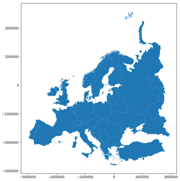
As we can see from the map, the projection is indeed centered to Helsinki as the 0-position of the x and y axis is located where Helsinki is positioned. Now the coordinate values are showing the distance from Helsinki (black point) to different directions (South, North, East and West) in meters.
Next, our goal is to calculate the distance from all countries to Helsinki. To be able to do that, we need to calculate the centroids for all the Polygons representing the boundaries of European countries.
- This can be done easily in Geopandas by using the
centroidattribute:
In [13]:
europe_borders_aeqd['centroid'] = europe_borders_aeqd.centroid
print(europe_borders_aeqd.head(2))
            TZID                                           geometry  \
0  Europe/Berlin  POLYGON ((-1057542.597130521 -493724.801682817...
1  Europe/Berlin  POLYGON ((-1216418.435359255 -1243831.63520634...

                                        centroid
0  POINT (-1057718.135423443 -492420.5658204998)
1  POINT (-1218235.216971495 -1242668.589667922)
Now we have created a new column called centroid that has the Point
geometries representing the centroids of each Polygon (in Azimuthal
Equidistant projection).
Next, we will calculate the distances between the country centroids and
Helsinki. For doing this, we could use iterrows() -function that we
have used earlier, but here we will demonstrate a more efficient
(faster) technique to go through all rows in (Geo)DataFrame by using
apply() -function.
The
apply()
-function can give a big boost in performance over the iterrows()
and it is the recommendable way of iterating over the rows in
(Geo)DataFrames. Here, we will see how to use that to calculate the
distance between the centroids and Helsinki.
- First, we will create a dedicated function for calculating the
distances called
calculate_distance():
In [14]:
def calculate_distance(row, dest_geom, src_col='geometry', target_col='distance'):
    """
    Calculates the distance between Point geometries.

    Parameters
    ----------
    dest_geom : shapely.Point
       A single Shapely Point geometry to which the distances will be calculated to.
    src_col : str
       A name of the column that has the Shapely Point objects from where the distances will be calculated from.
    target_col : str
       A name of the target column where the result will be stored.

    Returns
    -------

    Distance in kilometers that will be stored in 'target_col'.
    """

    # Calculate the distances
    dist = row[src_col].distance(dest_geom)

    # Convert into kilometers
    dist_km = dist / 1000

    # Assign the distance to the original data
    row[target_col] = dist_km
    return row
Here, the parameter row is used to pass the data from each row of
our GeoDataFrame into the function. Other paramaters are used for
passing other necessary information for using our function.
- Before using our function and calculating the distances between
Helsinki and centroids, we need to get the Shapely point geometry
from the re-projected Helsinki center point that we can pass to our
function (into the
dest_geom-parameter. We can use theloc-functionality to retrieve the value from specific index and column:
In [15]:
# Retrieve the geometry from Helsinki GeoDataFrame
helsinki_geom = helsinki.loc[0, 'geometry']
print(helsinki_geom)
POINT (0 0)
Now we are ready to use our function with apply(). When using the
function, it is important to specify the direction of iteration that
should be in our case specified with axis=1. This ensures that the
calculations are done row by row (instead of column-wise).
- When iterating over a DataFrame or GeoDataFrame, apply function is
used by following the format
GeoDataFrame.apply(name_of_your_function, param1, param2, param3, axis=1)- Notice that the first parameter is always the name of the function
that you want to use WITHOUT the parentheses. This will start
the iteration using the function you have created, and the values
of the row will be inserted into the
rowparameter / attribute inside the function (see above).
- Notice that the first parameter is always the name of the function
that you want to use WITHOUT the parentheses. This will start
the iteration using the function you have created, and the values
of the row will be inserted into the
In [16]:
# Calculate the distances using our custom function called 'calculate_distance'
europe_borders_aeqd = europe_borders_aeqd.apply(calculate_distance, dest_geom=helsinki_geom, src_col='centroid', target_col='dist_to_Hki', axis=1)
print(europe_borders_aeqd.head(10))
            TZID                                           geometry  \
0  Europe/Berlin  POLYGON ((-1057542.597130521 -493724.801682817...
1  Europe/Berlin  POLYGON ((-1216418.435359255 -1243831.63520634...
2  Europe/Berlin  POLYGON ((-1194521.638643212 -571726.459328880...
3  Europe/Berlin  POLYGON ((-1185933.276237431 -571780.052772927...
4  Europe/Berlin  POLYGON ((-1182416.219837205 -569097.571220089...
5  Europe/Berlin  POLYGON ((-1172799.400650826 -565749.438722840...
6  Europe/Berlin  POLYGON ((-1162805.427517967 -563558.434197176...
7  Europe/Berlin  POLYGON ((-1129053.540904054 -568388.469960322...
8  Europe/Berlin  POLYGON ((-1109126.532709598 -570899.989413469...
9  Europe/Berlin  POLYGON ((-703490.1465879162 -664009.791857452...

                                        centroid  dist_to_Hki
0  POINT (-1057718.135423443 -492420.5658204998)  1166.724332
1  POINT (-1218235.216971495 -1242668.589667922)  1740.207536
2   POINT (-1194210.78929945 -568987.1532380249)  1322.832487
3  POINT (-1185320.605845876 -571340.3134827727)  1315.832319
4  POINT (-1182191.163363772 -567293.7639830824)  1311.258236
5  POINT (-1175758.089721245 -564846.4759828373)  1304.399719
6  POINT (-1157868.191291224 -565162.3607219104)  1288.435968
7  POINT (-1124883.959682356 -567850.4028534379)  1260.086506
8   POINT (-1113376.309723986 -569037.768865205)  1250.364263
9   POINT (-703970.5591804661 -663710.575604432)   967.515517
Great! Now we have successfully calculated the distances between the Polygon centroids and Helsinki. 😎
- Let’s check what is the longest and mean distance to Helsinki from the centroids of other European countries:
In [17]:
# Calculat the maximum and average distance
max_dist = europe_borders_aeqd['dist_to_Hki'].max()
mean_dist = europe_borders_aeqd['dist_to_Hki'].mean()

print("Maximum distance to Helsinki is %.0f km, and the mean distance is %.0f km." % (max_dist, mean_dist))
Maximum distance to Helsinki is 3470 km, and the mean distance is 1177 km.
As we can see, the finns living in the North are fairly far away from all other European countries, as the mean distance to other countries is 1185 kilometers.
Notice: If you would like to calculate distances between multiple locations across the globe, it is recommended to use Haversine formula to do the calculations. Haversine package in Python provides an easy-to-use function for calculating these based on latitude and longitude values.
Summary
During this tutorial we have seen how to
1) define the coordinate reference system with a few different approaches, mainly by:
- specifying the coordinate reference system with crs dictionary e.g.
{'init': 'epsg:4326'} - specifying CRS with Proj4-string using PyCRS library:
pycrs.parser.from_epsg_code(4326).to_proj4() - specifying slightly less common CRS (Azimuthal Equidistant) with
Proj4-string using pyproj library:
pyproj.Proj(proj='aeqd', ellps='WGS84', datum='WGS84', lat_0=hki_lat, lon_0=hki_lon).srs - A fourth option that was not covered in the materials is to use a
library called
fionaand its functionfrom_epsg(). See documentation about this from here if you are interested. We also quickly introduced this in the previous tutorial.
2) reproject (transform) the geometries from crs to another using
the to_crs() -function in GeoPandas
3) calculate distances between locations and using apply()
-function to iterate over rows more efficiently than using
iterrows().